
I originally posted this at http://dtrace.org/blogs/brendan/2011/06/03/file-system-latency-part-5.
This is part 5 of File System Latency, a series on storage I/O performance from the application perspective (see parts 1, 2, 3 and 4). Previously I explained why disk I/O metrics may not reflect application performance, and how some file system issues may be invisible at the disk I/O level. I then showed how to resolve this by measuring file system latency at the application level using MySQL as an example, and measured latency from other levels of the operating system stack to pinpoint the origin.
The main tool I've used so far is DTrace, which is great for prototyping new metrics in production. In this post, I'll show what this can mean beyond DTrace, establishing file system latency as a primary metric for system administrators and application developers. I'll start by discussing the history for this metric on the Solaris operating system, how it's being used at the moment, and what is coming up next.
This is not just a pretty tool, but the culmination of years of experience (and pain) with file system and disk performance. I've explained this history a little below. To cut to the chase, see the Cloud Analytics and vfsstat sections.
A Little History
During the last five years, new observability tools have appeared on Solaris to measure file system latency and file system I/O. In particular these have targeted the Virtual File System (VFS) layer, which is the kernel (POSIX-based) interface for file systems (and was traced in part 4):
                  +---------------+
                  |  Application  |
                  |    mysqld     |
                  +---------------+
                   reads ^ | writes
                         | |
                         | |                  user-land
      -------------system calls---------------------------
                         | |                  kernel
                 +------------------+
        HERE --> |       VFS        |
                 +------------------+
                   ^ |         ^ |
                   | V         | V
               +--------+   +-------+
               |   ZFS  |   |  UFS  |  ...
               +--------+   +-------+
[...]
Outside of kernel engineering, the closest most of us got to VFS was in operating systems books, seen in diagrams like that above. It's been an abstract notion - not really a practical and observable component. This attitude has been changing with the release of DTrace (2003), which allows us to measure VFS I/O and latency directly, and fsstat(1M), a tool for file system statistics (2006).
Richard McDougall, Jim Mauro and I presented some DTrace-based tools to measure file system I/O and latency at the VFS layer in Solaris Performance and Tools (Prentice Hall, 2006), including vopstat (p118) and fsrw.d (p116). These and other VFS tracing scripts (fspaging.d, rfileio.d, rfsio.d, rwbytype.d) are in the DTraceToolkit (see the FS subdirectory).
fsstat(1M) was also developed in 2006 by Rich Brown to provide kstat-based VFS statistics (PSARC 2006/34) and added to Solaris. This tool is great, and since it is kstat-based it provides historic values with negligible performance overhead. (Bryan Cantrill later added DTrace probes to the kstat instrumentation, to form the fsinfo provider: PSARC 2006/196.) However, fsstat(1M) only provides operation and byte counts, not file system latency - which we really need.
For the DTrace book (Prentice Hall, 2011), Jim and I produced many new VFS scripts, covering Solaris, Mac OS X and FreeBSD. These are in the File Systems chapter (which is available as a PDF). While many of these did not report latency statistics, it is not difficult to enhance the scripts to do so, tracing the time between the "entry" and "return" probes (as was demonstrated via a one-liner in part 4).
DTrace has been the most practical way to measure file system latency across arbitrary applications, especially scripts like those in part 3. I'll comment briefly on a few more sources of performance metrics on Solaris: kstats, truss(1M), LatencyTOP, and application instrumentation.
kstats
Kernel statistics (kstats) is a "registry of metrics" (thanks Ben for the term) on Solaris, which provide the raw numbers for traditional observability tools including iostat(1M). While there are many thousands of kstats available, file system latency was not among them.
Even if you were a vendor whose job it was to build monitoring tools on top of Solaris, you can only use what the operating system gives you, hence the focus on disk I/O statistics from iostat(1M) or kstat. More on this in a moment (vfsstat).
truss, strace
You could attach system call tracers such as truss(1) or strace(1) to applications one-by-one to get latency from the syscall level. This would involve examining reads and writes and associating them back to file system-based file descriptors, along with timing data. However, the overhead of these tools is often prohibitive in production due to the way these tools work.
LatencyTOP
Another tool that could measure file system latency is LatencyTOP. This was released in 2008 by Intel to identify sources of desktop latency on Linux, and implemented by the addition of static trace points throughout the kernel. To see if DTrace could fetch similar data without kernel changes, I quickly wrote latencytop.d. LatencyTOP itself was ported to Solaris in 2009 (PSARC 2009/339):
LatencyTOP uses the Solaris DTrace APIs, specifically the following DTrace providers: sched, proc and lockstat.
While it isn't a VFS or file system oriented tool, its latency statistics do include file system read and write latency, presenting them as a "Maximum" and "Average". With these, it may be possible to identify instances of high latency (outliers), and increased average latency. Which is handy, but about all that is possible. To confirm that file system latency is directly causing slow queries, you'll need to use more DTrace like I did in part 3 to sum file system latency during query latency.
Applications
Application developers can instrument their own code as it performs file I/O, collecting high resolution timestamps to calculate file system latency metrics[1]. Because of this, they haven't needed DTrace, however they do need the foresight to have added these metrics before the application is in production. Too often I've been looking at a system where if we could restart the application with different options, then we could probably get the performance data we need. But restarting the application comes with serious cost (downtime), and can mean that the performance issue isn't visible again for hours or days (eg, memory growth/leak related). DTrace lets me get this data immediately.
That's not to say that DTrace is better than application-level metrics - it isn't. If the application already provides file system latency metrics, then use them. Running DTrace will add much more performance overhead than (well designed) application-level counters.
Check what the application provides before turning to DTrace.
I put this high up in the Strategy sections in the DTrace book, not only to avoid re-inventing the wheel, but since familiarization with application metrics is excellent context to build upon with DTrace.
[1] Well, almost. See the "CPU Latency" section in part 3, which is also true for application-level measurements. DTrace can inspect the kernel and differentiate CPU latency from file system latency, but as I said in part 3, you don't want to be running in a CPU latency state to start with.
MySQL
I've been using MySQL as an example application to investigate with DTrace. Apart from illustrating the technique, this may serve a second reason: a solution for systems with DTrace but no MySQL support for measuring file system latency. Recent versions of MySQL have provided the performance schema which can do this. Mark Leith posted a detailed article: Monitoring MySQL IO Latency with performance_schema, writing:
filesystem latency can be monitored from the current MySQL 5.5 GA version, with performance schema, on all platforms.
In part 3 I thought it would need version 5.6 to do this, but Mark has demonstrated this on 5.5 GA. This is good news if you are on MySQL 5.5 GA or later, and are running with the performance-schema option.
The DTrace story doesn't quite end here. I'll save this for a separate post as it's more about the MySQL performance schema than the file system latency metric.
What's Happening Now
I'm regularly using DTrace to identify issues of high file system latency, and to quantify how much it is affecting application performance. This is for cloud computing environments, where multiple tenants are sharing a pool of disks, and where disk I/O statistics from iostat(1M) look more alarming than reality (reasons why this can happen are explained in part 1).
The most useful scripts I'm using include those in part 3 to measure latency from within MySQL, and also because these scripts can be run by the customer. Most of the time they show that the file system is performing great, and returning out of DRAM cache (thanks to our environment). This leads the investigation to other areas, narrowing the scope to where the issue really is and saving time skipping where it isn't.
I've identified real disk based issues as well (which are fortunately rare) which when traced as file system latency show that the application really is affected. Again, this saves time, as knowing that there is a file system issue to investigate is a much better position than knowing that there might be one.
Tracing file system latency has worked best from two locations:
Application layer: as demonstrated in part 3, which provides application context to identify if the issue is real (synchronous to workload) and what is affected (workload attributes). The key example from that post was mysqld_pid_fslatency_slowlog.d, which printed the total file system latency along with the query latency - so that slow queries could be immediately identified as file system-based or not.
VFS layer: as demonstrated in part 4, which allows all applications to be traced simultaneously regardless of their I/O code-path. Since these trace inside the kernel, the scripts are unable to be run by customers in the cloud computing environment (zones), as the fbt provider is not available.
For the rare times that there is high file system latency, I'll dig down deeper into the kernel stack to pinpoint the location: tracing the specific file system type (ZFS, UFS, ...), and disk device drivers, as shown in part 4 and chapters 4 and 5 of the DTrace book. This includes using several custom fbt provider-based DTrace scripts, which are fairly brittle as they trace a specific kernel version.
What's Next
File system latency has become so important that examining it interactively via DTrace scripts is not enough. Many people do use remote monitoring tools (eg, munin) to fetch statistics for graphing, and it's not straight-forward to run these DTrace scripts 24x7 to feed remote monitoring. And those tools would be better to show the full distribution of latency, such as with a heat map, and not just a line graph of the average latency per-second.
At Joyent we've been developing solutions to these on the latest version of our operating system, SmartOS (which is Illumos based). These solutions include vfsstat(1M) and the file system latency instrumentation in Cloud Analytics.
vfsstat(1M)
For a disk I/O summary, iostat(1M) does do a good job (using -x for the extended columns). The main issue is that from an application perspective we'd like the statistics to be measured closer to the app, such as in the VFS level.
vfsstat(1M) is a new tool developed by Bill Pijewski of Joyent to do this. You can think of it as an iostat(1M)-like tool for the VFS level, breaking down by smartmachine (zone) instead of by-disk. He showed it in a recent blog post here on dtrace.org. Sample output:
$ vfsstat 1
  r/s   w/s  kr/s  kw/s ractv wactv read_t writ_t  %r  %w   d/s  del_t zone
  2.5   0.1   1.5   0.0   0.0   0.0    0.0    2.6   0   0   0.0    8.0 06da2f3a (437)
1540.4   0.0 195014.9   0.0   0.0   0.0    0.0    0.0   3   0   0.0    0.0 06da2f3a (437)
1991.7   0.0 254931.5   0.0   0.0   0.0    0.0    0.0   4   0   0.0    0.0 06da2f3a (437)
1989.8   0.0 254697.0   0.0   0.0   0.0    0.0    0.0   4   0   0.0    0.0 06da2f3a (437)
1913.0   0.0 244862.7   0.0   0.0   0.0    0.0    0.0   4   0   0.0    0.0 06da2f3a (437)
^C
Rather than the VFS operation counts shown by fsstat(1M), vfsstat(1M) shows resulting VFS performance, including the average read I/O time ("read_t"). And unlike iostat(1M), if vfsstat(1M) is showing an increase in average latency then you know that applications have suffered.
If vfsstat(1M) does identify high latency, the next question is to check if sensitive code-paths have suffered (the "synchronous component of the workload" requirement), which can be identified using the pid provider. An example of this was the mysqld_pid_fslatency_slowlog.d script in part 3, which expressed total file system I/O latency next to query time.
vfsstat(1M) can be a handy tool to run before reaching for DTrace, as it is using kernel statistics (kstats) that are essentially free to use (already maintained and active), and can be run as a non-root user.
kstats
A new class of kstats were added for vfsstat(1M), called "zone_vfs". Listing them:
$ kstat zone_vfs
module: zone_vfs                        instance: 437
name:   06da2f3a-752c-11e0-9f4b-07732c  class:    zone_vfs
        100ms_ops                       107
        10ms_ops                        315
        1s_ops                          19
        crtime                          960767.771679531
        delay_cnt                       2160
        delay_time                      16925
        nread                           4626152694
        nwritten                        78949099
        reads                           7492345
        rlentime                        27105336415
        rtime                           21384034819
        snaptime                        4006844.70048824
        wlentime                        655500914122
        writes                          277012
        wtime                           576119455347
Apart from the data behind the vfsstat(1M) columns, there are also counters for file system I/O with latency greater than 10 ms (10ms_ops), 100 ms (100ms_ops), and 1 second (1s_ops). While these counters have coarse latency resolution, they do provide a historic summary of high file system latency since boot. This may be invaluable for diagnosing a file system issue after the fact, if it wasn't still happening for DTrace to see live, and if remote monitoring of vfsstat(1M) wasn't active.
Monitoring
vfsstat(1M) can be used as an addition to remote monitoring tools (like munin) which currently graph disk I/O statistics from iostat(1M). This not just provides sysadmins with historical graphs, but it also can provide others without root and DTrace access to observe VFS performance, including application developers and database administrators.
Modifying tools that already process iostat(1M) to also process vfsstat(1M) should be a trivial exercise. vfsstat(1M) also supports the -I option to prints absolute values, so that this could be executed every few minutes by the remote monitoring tool and averages calculated after the fact (without needing to leave it running):
$ vfsstat -Ir
r/i,w/i,kr/i,kw/i,ractv,wactv,read_t,writ_t,%r,%w,d/i,del_t,zone
6761806.0,257396.0,4074450.0,74476.6,0.0,0.0,0.0,2.5,0,0,0.0,7.9,06da2f3a,437
I used -r as well to print the output in comma-separated format, to make it easier to parse by monitoring software.
man page
Here are some exerpts, showing the other available switches and column definitions:
SYNOPSIS
     vfsstat [-hIMrzZ] [interval [count]]

DESCRIPTION
     The  vfsstat utility reports a summary of VFS read and write
     activity per zone.  It first prints all activity since boot,
     then reports activity over a specified interval.

     When  run  from  a non-global zone (NGZ), only activity from
     that NGZ can be observed.  When run from a the  global  zone
     (GZ),  activity  from  the  GZ  and  all  other  NGZs can be
     observed.
[...]
OUTPUT
     The vfsstat utility reports the following information:
         r/s  reads per second
         w/s  writes per second
         kr/s kilobytes read per second
         kw/s kilobytes written per second
         ractv     average number of read operations actively being
                   serviced by the VFS layer
         wactv     average number of write operations actively being
                   serviced by the VFS layer
         read_t    average VFS read latency
         writ_t    average VFS write latency
         %r   percent of time there is a VFS read operation
              pending
         %w   percent of time there is a VFS write operation
              pending
         d/s  VFS operations per second delayed by the ZFS I/O
              throttle
         del_t     average ZFS I/O throttle delay, in microseconds
OPTIONS
     The following options are supported:
     -h   Show help message and exit
     -I   Print results per  interval,  rather  than  per  second
     (where      applicable)
     -M   Print results in MB/s instead of KB/s
     -r   Show results in a comma-separated format
     -z   Hide zones with no VFS activity
     -Z   Print results for all zones, not just the current zone
[...]
Similar to how iostat(1M)'s %b (percent busy) metric works, the vfsstat(1M) %r and %w columns show the percentages of time that read or write operations were active. Once they hit 100% this only means that 100% of the time something was active - not that there is no more headroom to accept more I/O. It's the same for iostat(1M)'s %b - disk devices may accept additional concurrent requests even though they are already running at 100% busy.
I/O throttling
The default vfsstat(1M) output includes columns (d/s, del_t) to show the performance effect of I/O throttling - another feature by Bill that manages disk I/O in a multi-tenant environment. I/O throttle latency will be invisible at the disk level, like those other types described in part 2. And it is very important to observe, as file system latency issues could now simply be I/O throttling preventing a tenant from hurting others. Since it's a new latency type, I'll illustrate it here:
                   +-------------------------------+
                   |  Application                  |
                   |    mysqld                     |
                   +-------------------------------+
                      I/O |    I/O latency     ^ I/O
                  request |  <-------------->  | completion
                          |                    |
       ----------------------------------------------------
                          |                    |   <-- vfsstat(1M)
                          |                    |
          +-------------------------------------------+
          |  File System  |                    |      |
          |               |  I/O throttling    |      |
          |               X-------------->.    |      |
          |                               |I/O |      |
          |                               |wait|      |
          |                               V    |      |
          +-------------------------------------------+
                                          |    |
                                          |    |   <-- iostat(1M)
                                         .------.
                                         `------'
                                         | disk |
                                         `------'
As pictured here, the latency for file system I/O could be dominated by I/O throttling wait time, and not the time spent waiting on the actual disk I/O.
Averages
vfsstat(1M) is handy for some roles, such as an addition to remote monitoring tools that already handle iostat(1M)-like output. However, as a summary of average latency, it may not identify issues with the distribution of I/O. For example, if most I/O were fast with a few very slow I/O (outliers), the average may hide the presence of the few slow I/O. This is an issue we've encountered before, and solved using a 3rd dimension to show the entire distribution over time as a heat map. We've done this for file system latency in Cloud Analytics.
Cloud Analytics
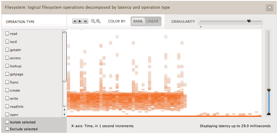
As I discussed in the MySQL Query Latency post, there can be interesting patterns seen over time that are difficult to visualize at the text-based command line. This is something that we are addressing with Cloud Analytics (videos), using heat maps to display file system latency. This is done for all applications and file sytems, by tracing in the kernel at the VFS level. Here is an example:
Time is the x-axis, file system I/O latency is the y-axis, and the number of I/O at each pixel is represented by color saturation (z-axis). The pixels are deliberately drawn large so that their x and y ranges will sometimes span multiple I/O, allowing various shades to be picked and patterns revealed.
This heatmap is showing a cloud node running MySQL 5.1.57, which was under a steady workload from sysbench. Most of the file system I/O is returning so fast it has been grouped in the first pixel at the bottom of the heat map, which represents the lowest latency.
Outliers
I/O with particularly high latency will be shown at the top of the heat map. The example above shows a single outlier at the top. This was clicked, revealing details below the heat map. It was a single ZFS I/O with latency between 278 and 286 ms.
This visualization makes identifying outliers trivial - outliers which can cause problems and can be missed when considering latency as an average. Finding outliers was also possible using the mysqld_pid_fslatency.d script from part 3; this is what an outlier with a similar latency range looks like from that script:
  read
           value  ------------- Distribution ------------- count
            1024 |                                         0
            2048 |@@@@@@@@@@@                              2926
            4096 |@@@@@@@@@@@@@@@@                         4224
            8192 |@@@@@@@@                                 2186
           16384 |@@@@@                                    1318
           32768 |                                         96
           65536 |                                         3
          131072 |                                         5
          262144 |                                         0
          524288 |                                         0
         1048576 |                                         0
         2097152 |                                         1
         4194304 |                                         3
         8388608 |                                         2
        16777216 |                                         1
        33554432 |                                         1
        67108864 |                                         0
       134217728 |                                         0
       268435456 |                                         1
       536870912 |                                         0
Consider taking this distribution and plotting it as a single column in the heat map. Do this every second, displaying them across the x-axis. This is what Cloud Analytics does, which also uses DTrace to efficiently collect and aggregate the data in-kernel as the distribution before passing the summary to user-land. Cloud Analytics also uses a higher resolution distribution than the power-of-2 shown here: it uses Log/linear quantization which Bryan added to DTrace for this very reason.
The mysqld_pid_fslatency.d script did show a separate distribution for reads and writes; this is also possible in Cloud Analytics, which can measure details as an extra dimension.
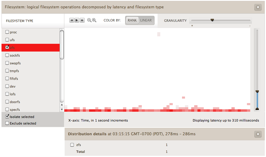
4th dimension
The dataset can include another attribute to breakdown the data, which in the example above was the file system type. This is like having a 4th dimension in the dataset - potentially very useful, but tricky to visualize. We've used different color hues for the elements in that dimension, which can be selected by clicking the list on the left:
This shows writes in blue and fsyncs in green. These were also shown in isolation from the other operation types to focus on their details, and the y-axis has been zoomed to show finer details: latency from 0 to 0.4 ms.
This heat map also shows that that the distribution has detail across the latency axis: the fsyncs mostly grouped into two bands, and the writes were usually grouped into one lower latency band, but sometimes split into two. This split happened twice, for about 10 to 20 seconds each time, appearing as blue "arches". The higher band of latency is only about 100 microseconds slower - so it's interesting, but probably isn't an issue.
Time-based patterns
The x-axis, time, reveals patterns when the write latency changes second-by-second: seen above by the blue "arches". These would be difficult to spot at the command line; I could adjust the mysqld_pid_latency.d script to output the distribution every second - but I would need to read hundreds of pages of text-based distributions to comprehend the pattern seen in the above heat map.
This behavior was something I just discovered (I happen to be benchmarking MySQL for a different reason), and can't offer a explanation for this yet with certainty. Now that I know this behavior exists and the latency cost, I can decide if it is worth investigating further (with DTrace), or if there are larger latency issues to work on instead.
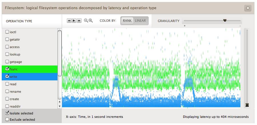
Here is another time-based pattern to consider, this time it's not MySQL:

It's iozone's auto mode.
iozone is performing numerous write and read tests, stepping up the file size and the record size of the I/O. The resulting I/O latency can be seen to creep up as the record size is increased for the runs, and reset again for the next run.
Other breakdowns
The screenshots I've used showed file system latency by file system, and by operation type. Here is the current list of possible breakdowns:
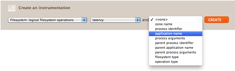
Since this is tracing at the VFS level, it still has application context allowing the application name and arguments to be examined.
Context
So far this is just showing I/O latency at the VFS level. If you've read my previous posts in this series, you'll know that this solves many problems but not all problems. It is especially good at identifying outliers, and for illustrating the full distribution, not just the average. However, having application (eg, MySQL) context lets us take it a step further, expressing file system latency as a portion of the application request time. This was demonstrated by the mysqld_pid_fslatency_slowlog.d script in part 3, which provides a metric that can measure and prove that file system latency was hurting the application's workload, and exactly by how much.
And more
Cloud Analytics can do (and will do) a lot more than just file system latency. See Dave Pacheco's blog (who is the lead engineer) for future posts. We'll also both be giving a talk at OSCONdata 2011 about it titled Design and Implementation of a Real-Time Cloud Analytics Platform.
For more background on these type of visualizations, see my ACMQ/CACM article on visualizing system latency, which focused on NFS latency (still a file system) and included other interesting patterns.
Reality check
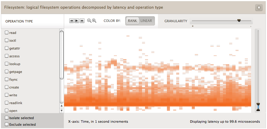
Interesting patterns like those above sometimes happen, but the distributions are more often mundane (at first glance). I'll finish by demonstrating this with a simple workload (which was also shown in the first screenshot in this post); A 1 Gbyte file is read randomly until it has been entirely cached:
About midway (60%) across the heat map (x-axis, time) the file became fully cached in DRAM. The left side shows three characteristics:
- A line at the bottom of the heat map, showing very fast file system I/O. These are likely to be DRAM cache hits (more DTrace could confirm if needed).
- A "cloud" of latency from about 3 to 10 ms. This is likely to be random disk I/O.
- Vertical spikes of latency, about every 5 seconds. This is likely evidence of some I/O queueing (serializing) behind an event, such as a file system flush. (More DTrace, like that used in part 4, can be used to identify the exact reason.)
This is great. Consider again what would happen if this was a line graph instead that showed average latency per second. All of these interesting details would be squashed into a single line, averaging both DRAM cache latency and disk I/O latency together.
Zooming in vertically on the right hand side reveals the latency of the DRAM hits:
This shows the distribution of the file system DRAM cache hits. The y-axis scale is now 100 microseconds (0.1 ms) - this extrordinary resolution made possible by both DTrace and Bryan's recent llquantize() addition.
Most of the latency is at the bottom of the distribution. In this case, the default rank-based palette (aka "false color palette") has emphasised the pattern in the higher latency ranges. It does this in an unusual but effective way: it applies the palatte evenly across a list of heat map elements sorted (ranked) by their I/O count, so that the full spectrum is used to emphasize details. There the I/O count affects the pixel rank, and the saturation is based on that rank. But the saturation isn't proportional: a pixel that is a little bit darker may span 10x the I/O.
Basing the saturation on the I/O count directly is how the linear-based palette works, which may not use every possible shade, but the shades will be correctly proportional. The "COLOR BY" control in Cloud Analytics allows this palette to be selected:
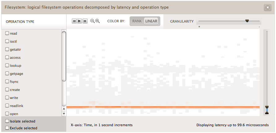
While the linear palette washes out finer detals, it's better at showing where the bulk of the I/O were - here the darker orange line of lower latency.
Conclusion
File system latency has become an essential metric for understanding application performance, with increased functionality and caching of file systems leaving disk-level metrics confusing and incomplete. Various DTrace-based tools have been created to measure file system latency, with the most effective expressing it as a synchronous component of the application workload: demonstrated here by the sum of file system latency during a MySQL query. I've been using these tools for several months, solving real world performance issues in a cloud computing environment.
To allow file system latency to be more easily observed, a new command line tool has been developed, vfsstat(1M), which reports iostat(1M)-like metrics for the VFS level and can be consumed by remote monitoring tools. To allow it to be examined in greater detail, it has also been added to Joyent's Cloud Analytics as a heat map, with various breakdowns possible. If needed, DTrace at the command-line can be used to inspect latency event-by-event, and at any layer of the operating system stack from the application interface to the kernel device drivers - to pinpoint the origin.