

I originally posted this at http://blogs.sun.com/brendan/entry/heat_map_analytics.
I've been recently posting screenshots of heat maps from Analytics: the observability tool shipped with the Sun Storage 7000 series.
These heat maps are especially interesting, which I'll describe here in more detail.
Introduction
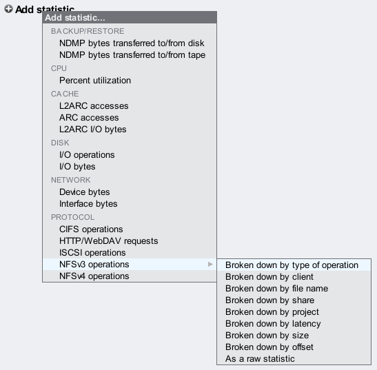
To start with, when you first visit Analytics you have an empty worksheet and need to add statistics to plot. Clicking on the plus icon next to "Add statistic" brings up a menu of statistics, as shown on the right.
I've clicked on "NFSv3 operations" and a sublist of possible breakdowns are shown. The last three (not including "as a raw statistic") are represented as heat maps. Clicking on "by latency" would show "NFSv3 operations by latency" as a heat map. Great.
But it's actually much more powerful than it looks. It is possible to drill down on each breakdown to focus on behavior of interest. For example, latency may be more interesting for read or write operations, depending on the workload. If our workload was performing synchronous writes, we may like to see the NFS latency heat map for 'write' operations separately, which we can do with Analytics.
To see an example of this, I've selected "NFS operations by type of operation", then selected 'write', then right-clicked on the "write" text to see the next breakdowns that are possible:

This menu is also visible by clicking the drill icon (3rd from the right) to drill down further.
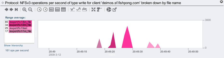
By clicking on latency, it will now graph "NFSv3 operations of type write broken down by latency". So these statistics can be shown in whatever context is most interesting. Perhaps I want to see NFS operations from a particular client, or for a particular file. Here are NFSv3 writes from the client 'deimos', showing the filenames that are being written:
Awesome. Behind the scenes, DTrace is building up dynamic scripts to fetch this data. We just click the mouse.
This was important to mention – the heat maps I'm about to demonstrate can be customized very specifically, by type of operation, client, filename, etc.
Sequential reads
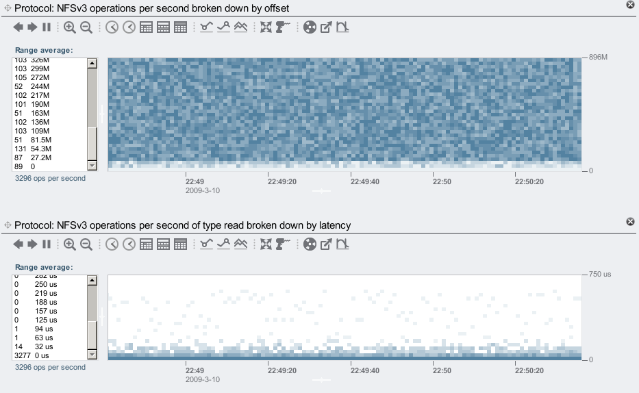
I'll demonstrate heat maps at the NFS level by running the /usr/bin/sum command on a large file a few times, and letting it run longer each time before hitting Ctrl-C to cancel it. The sum command calculates a file's checksum, and does so by sequentially reading through the file contents. Here is what the three heat maps from Analytics shows:
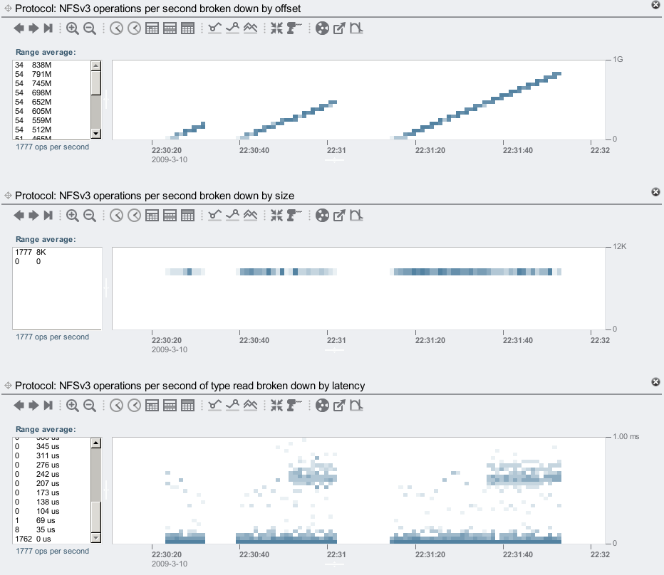
The top heat map of offset clearly shows the client's behavior, the stripes show sequential I/O. The blocks show the offsets of the read operations as the client creeps through the file. I mounted the client using forcedirectio, so that NFS would not cache on the file contents on the client, and would be forced to keep reading the file each time.
The middle heat map shows the size of the client I/O requests. This shows the NFS client is always requesting 8 Kbyte reads. The bottom heat map shows NFS I/O latency. Most of the I/O was between 0 and 35 microseconds, but there are some odd clouds of latency on the 2nd and 3rd runs.
These latency clouds would be almost invisible if a linear color scheme was used. These heat maps use false color to emphasize detail. The left panel showed that on average there were 1771 ops/sec faster than 104 us (adding up the numbers), and that the entire heat map averaged at 1777 ops/sec; this means that the latency clouds (at about 0.7 ms) represent 0.3% of the I/O. The false color scheme makes them clearly visible, which is important for latency heat maps, as these slow outliers can hurt performance, even though they are relatively infrequent.
For those interested in more detail, I've included a couple of extra screenshots to explain this further:
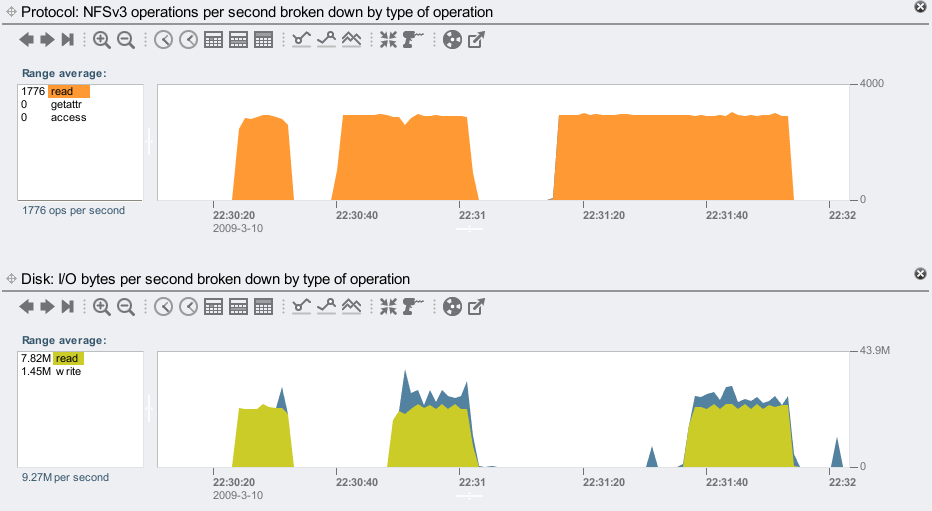
- Screenshot 1: NFS operations and disk throughput. From the top graph, it's clear how long I left the sum command running each time. The bottom graph of disk I/O bytes shows that the file I was checksumming had to be pulled in from disk for the entire first run, but only later in the second and third runs. Correspond the times to the offset heat map above. The 2nd and 3rd runs are reading data that is now cached, and doesn't need to be read from disk.
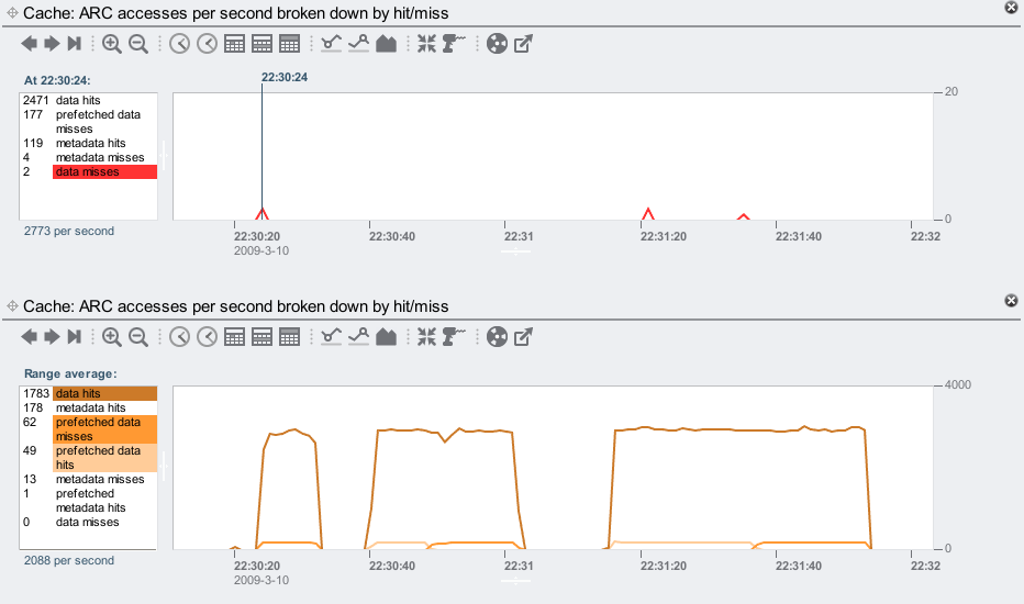
- Screenshot 2: ARC hits/misses. This shows what the ZFS DRAM cache is doing (which is the ARC: the Adaptive Replacement Cache). I've shown the same statistic twice, so that I can highlight breakdowns separately. The top graph shows a data miss at 22:30:24, which triggers ZFS to prefetch the data (since ZFS detects that this is a sequential read). The bottom graph shows data hits are kept high, thanks to ZFS prefetch, and ZFS prefetch in operation: the "prefetched data misses" shows requests triggered by prefetch that were not already in the ARC, and read from disk; and the "prefetched data hits" shows prefetch requests that were already satisfied by the ARC. The latency clouds correspond to the later prefetch data misses, where some client requests are arriving while prefetch is still reading from disk, and are waiting for that to complete.
Random reads
While the rising stripes of a sequential workload are clearly visible in the offset heat map, random workloads are also easily identifiable:
The NFS operations by offset shows a random and fairly uniform pattern, which matches the random I/O I now have my client requesting. These are all hitting the ZFS DRAM cache, and so the latency heat map shows most responses in the 0 to 32 microsecond range.
Checking how these known workloads look in Analytics is valuable, as when we are faced with the unknown we know what to look for.
Disk I/O
The heat maps above demonstrated Analytics at the NFS layer; Analytics can also trace these details at the back-end: what the disks are doing, as requested by ZFS. As an example, here is a sequential disk workload:

The heat maps aren't as clear as they are at the NFS layer, as now we are looking at what ZFS decides to do based on our NFS requests.
The sequential read is mostly reading from the first 25 Gbytes of the disks, as shown in the offset heat map. The size heat map shows ZFS is doing mostly 128 Kbyte I/Os, and the latency heat map shows the disk I/O time is often about 1.20 ms, and longer.
Latency at the disk I/O layer doesn't directly correspond to client latency – it depends on the type of I/O. Asynchronous writes and prefetch I/O won't necessarily slow the client, for example.
Vertical Zoom
There is a way to zoom these heat maps vertically. Zooming horizontally is obvious (the first 10 buttons above each heat map do that by changing the time range), but the vertical zoom isn't so obvious. It is documented in the online help, I just wanted to say here that it does exist. In a nutshell: click the outliers icon (last on the right) to switch outlier elimination modes (5%, 1%, 0.1%, 0.01%, none), which often will do what you want (by zooming to exclude a percentage of outliers); otherwise left click a low value in the left panel, shift click a high value, then click the outliers icon.
Overheads
As mentioned earlier, these heat maps use optimal resolutions at different ranges to conserve disk space, while maintaining visual resolution. They are also saved on the system disks, which have compression enabled. Still, when recording this data every second, 24 hours a day, the disk space can add up. Check their disk usage by going to Analytics->Datasets and clicking the "ON DISK" title to sort by size:

The size is listed before compression, so the actual consumed bytes is lower. These datasets can be suspended by clicking the power button, which is handy if you'd like to keep interesting data but not continue to collect new data.
Playing around...
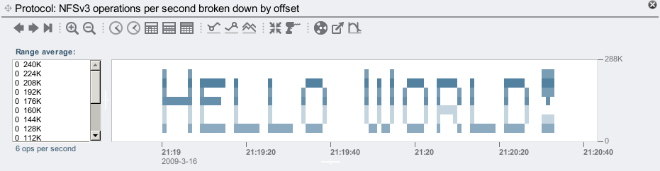
While using these heat maps we noticed some unusual and detailed plots. Bryan and I starting wondering if it were possible to generate artificial workloads that plotted arbitrary patterns, such as spelling out words in 8 point text. This would be especially easy for the offset heat map at the NFS level, since the client requests the offsets, we just need to write a program to request reads or writes to the offsets we want. Moments after this idea, Bryan and I were furiously coding to see who could finish it first (and post comical messages to each other). Bryan won, after about 10 minutes. Here is an example:
Awsome, dude! ... (although that wasn't the first message we printed ... when I realized Bryan was winning, I logged into his desktop, found the binary he was compiling, and posted the first message to his screen before he had finished writing the software. However my message appeared as: "BWC SnX" (Bryan's username is "bmc".) Bryan was looking at the message, puzzled, while I'm saying "it's upside down – your program prints upside down!")
I later modified the program to work for the size heat maps as well, which was easy as the client requests it. But what about the latency heat maps? Latency isn't requested, it depends on many factors. For reads, it depends on whether the data is cached, and if not, whether it is on a flash memory based read cache (if one is used), and if not, then it depends on how much disk head seek and rotation time it takes to pull it in, which varies depending on the previous disk I/O. Maybe this can't be done...
Actually, it can be done. Here is all three:
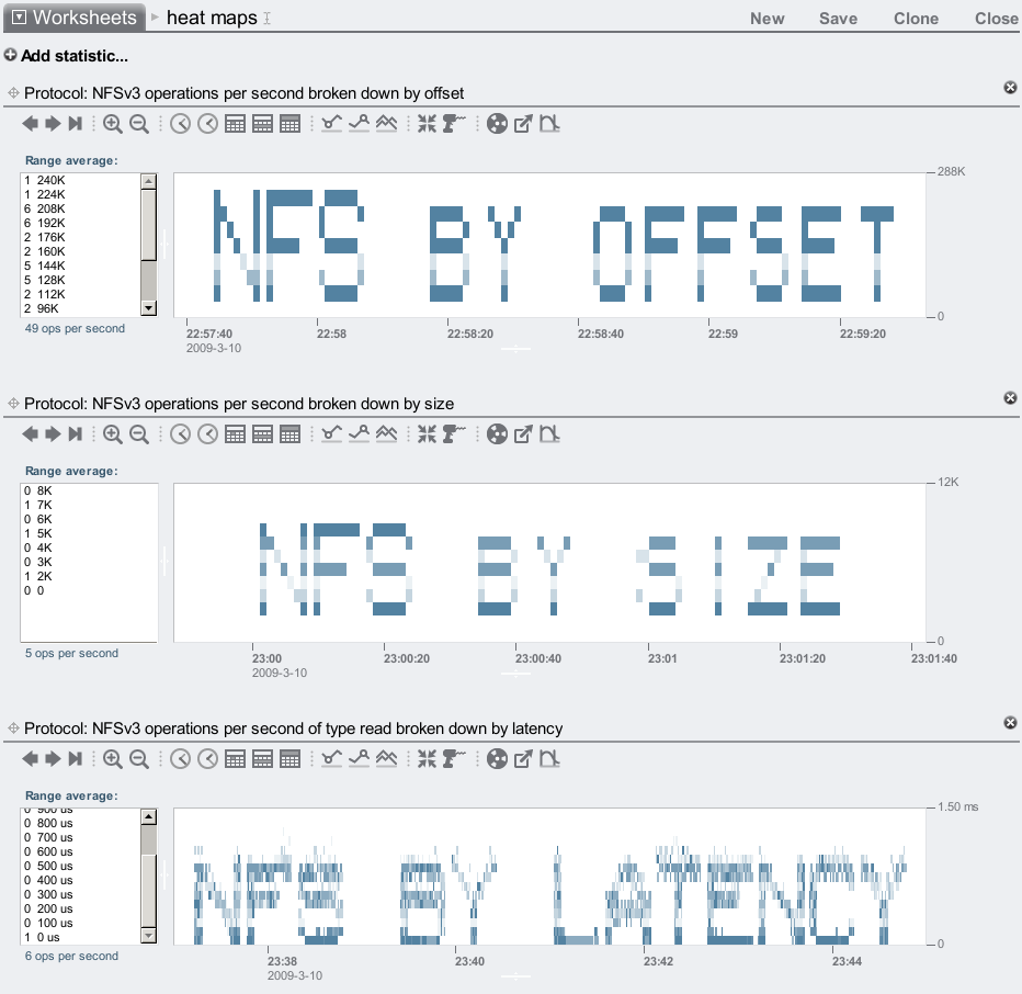
Ok, the latency heat map looks a bit fuzzy, but this does work. I could probably improve it if I spent more than 30 mins on the code, but I have plenty of actual work to do.
I got the latency program to work by requesting data which was cached in DRAM, of large increasing sizes. The latency from DRAM is consistent and relative to the size requested, so by calling reads with certain large I/O sizes I can manufacture a workload with the latency I want (close to). The client was mounted forcedirectio, so that every read caused an NFS I/O (no client caching.)
If you are interested in the client programs that injected these workloads, they are provided here (completely unsupported) for your entertainment: offsetwriter.c, sizewriter.c and latencywriter.c. If you don't have a Sun Storage 7000 series product to try them on, you can try the fully functional VMware simulator (although they may need adjustments to compensate for the simulator's slower response times).
Summary
Heat maps are an excellent visual tool for analyzing data, and identifying patterns that would go unnoticed via text based commands or plain graphs. Some may remember Richard McDougall's Taztool, which used heat maps for disk I/O by offset analysis, and was very useful at the time (I reinvented it later for Solaris 10 with DTraceTazTool).
Analytics takes heat maps much further:
- visibility of different layers of the software stack: disk I/O, NFS, CIFS, ...
- drilldown capabilities: for a particular client or file only, ...
- I/O by offset, I/O by size and I/O by latency
- can archive data 24x7 in production environments
- optimal disk storage
With this new visibility, heat maps are illuminating numerous performance behaviors that we previously didn't know about and some we still don't yet understand – like the Rainbow Pterodactyl. DTrace has made this data available for years, Analytics is making it easy to see.