Linux Extended BPF (eBPF) Tracing Tools


My BPF Perf Tools book
This page shows examples of performance analysis tools using enhancements to BPF (Berkeley Packet Filter) which were added to the Linux 4.x series kernels, allowing BPF to do much more than just filtering packets. These enhancements allow custom analysis programs to be executed on Linux dynamic tracing, static tracing, and profiling events.
The main and recommended front-ends for BPF tracing are BCC and bpftrace: BCC for complex tools and daemons, and bpftrace for one-liners and short scripts. If you are looking for tools to run, try BCC then bpftrace. If you want to program your own, start with bpftrace, and only use BCC if needed. I've ported many of my older tracing tools to both BCC and bpftrace, and their repositories provide over 100 tools between them. I also developed over 100 more for my book: BPF Performance Tools: Linux System and Application Observability.
eBPF tracing is suited for answering questions like:
- Are any ext4 operations taking longer than 50 ms?
- What is run queue latency, as a histogram?
- Which packets and apps are experiencing TCP retransmits? Trace efficiently (without tracing send/receive).
- What is the stack trace when threads block (off-CPU), and how long do they block for?
eBPF can also be used for security modules and software defined networks. I'm not covering those here (yet, anyway). Also note: eBPF is often called just "BPF", especially on lkml.
Table of contents:
On this page I'll describe eBPF, the front-ends, and demonstrate some of the tracing tools I've developed.
1. Screenshot
Starting with a screenshot, here's an example of tracing and showing block (disk) I/O as a latency heat map:
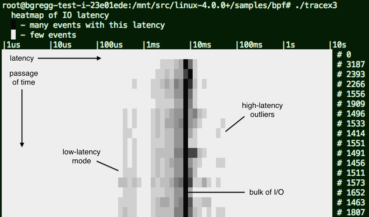
I added some annotations to that screenshot. If you are new to this visualization, see my page on latency heat maps.
This uses kernel dynamic tracing (kprobes) to instrument functions for the issue and completion of block device I/O. Custom eBPF programs execute when these kprobes are hit, which record timestamps on the issue of I/O, fetch them on completion, calculate the delta time, and then store this in a log 2 histogram. The user space program reads this histogram array periodically, once per second, and draws the heat map. The summarization is all done in kernel context, for efficiency.
2. One Liners
Useful one-liners using the bcc (eBPF) tools:
Single Purpose Tools
# Trace new processes:
execsnoop

# Trace file opens with process and filename:
opensnoop

# Summarize block I/O (disk) latency as a power-of-2 distribution by disk:
biolatency -D

# Summarize block I/O size as a power-of-2 distribution by program name:
bitesize

# Trace common ext4 file system operations slower than 1 millisecond:
ext4slower 1

# Trace TCP active connections (connect()) with IP address and ports:
tcpconnect

# Trace TCP passive connections (accept()) with IP address and ports:
tcpaccept

# Trace TCP connections to local port 80, with session duration:
tcplife -L 80

# Trace TCP retransmissions with IP addresses and TCP state:
tcpretrans

# Sample stack traces at 49 Hertz for 10 seconds, emit folded format (for flame graphs):
profile -fd -F 49 10

# Trace details and latency of resolver DNS lookups:
gethostlatency

# Trace commands issued in all running bash shells:
bashreadline
Multi Tools: Kernel Dynamic Tracing
# Count "tcp_send*" kernel function, print output every second:
funccount -i 1 'tcp_send*'

# Count "vfs_*" calls for PID 185:
funccount -p 185 'vfs_*'

# Trace file names opened, using dynamic tracing of the kernel do_sys_open() function:
trace 'p::do_sys_open "%s", arg2'

# Same as before ("p:: is assumed if not specified):
trace 'do_sys_open "%s", arg2'

# Trace the return of the kernel do_sys_open() funciton, and print the retval:
trace 'r::do_sys_open "ret: %d", retval'

# Trace do_nanosleep() kernel function and the second argument (mode), with kernel stack traces:
trace -K 'do_nanosleep "mode: %d", arg2'

# Trace do_nanosleep() mode by providing the prototype (no debuginfo required):
trace 'do_nanosleep(struct hrtimer_sleeper *t, enum hrtimer_mode mode) "mode: %d", mode'

# Trace do_nanosleep() with the task address (may be NULL), noting the dereference:
trace 'do_nanosleep(struct hrtimer_sleeper *t, enum hrtimer_mode mode) "task: %x", t->task'

# Frequency count tcp_sendmsg() size:
argdist -C 'p::tcp_sendmsg(struct sock *sk, struct msghdr *msg, size_t size):u32:size'

# Summarize tcp_sendmsg() size as a power-of-2 histogram:
argdist -H 'p::tcp_sendmsg(struct sock *sk, struct msghdr *msg, size_t size):u32:size'

# Frequency count stack traces that lead to the submit_bio() function (disk I/O issue):
stackcount submit_bio

# Summarize the latency (time taken) by the vfs_read() function for PID 181:
funclatency -p 181 -u vfs_read
Multi Tools: User Level Dynamic Tracing
# Trace the libc library function nanosleep() and print the requested sleep details:
trace 'p:c:nanosleep(struct timespec *req) "%d sec %d nsec", req->tv_sec, req->tv_nsec'

# Count the libc write() call for PID 181 by file descriptor:
argdist -p 181 -C 'p:c:write(int fd):int:fd'

# Summarize the latency (time taken) by libc getaddrinfo(), as a power-of-2 histogram in microseconds:
funclatency.py -u 'c:getaddrinfo'
Multi Tools: Kernel Static Tracing
# Count stack traces that led to issuing block I/O, tracing its kernel tracepoint:
stackcount t:block:block_rq_insert
Under construction...
Multi Tools: User Statically Defined Tracing (USDT)
# Trace the pthread_create USDT probe, and print arg1 as hex:
trace 'u:pthread:pthread_create "%x", arg1'
Under construction...
These one-liners demonstrate various capabilities of bcc/eBPF. You can also print these out as a cheatsheet.
3. Presentation
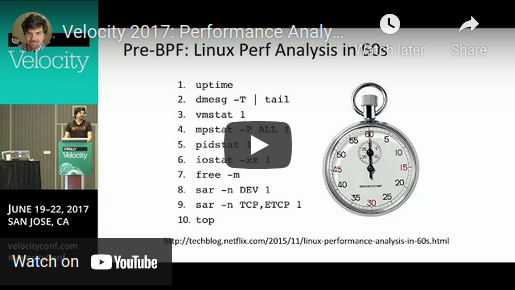
My recent talk on eBPF tracing tools at O'Reilly Velocity 2017 (slideshare, youtube, PDF).
Other presentations:
- BPF: Tracing and More, by Brendan Gregg at linux.conf.au 2017 (slideshare, youtube, PDF).
- Linux 4.x Tracing Tools: Using BPF Superpowers, by Brendan Gregg at USENIX LISA 2016 (slideshare, youtube, PDF).
- My Give me 15 minutes and I'll change your view of Linux tracing demo from LISA 2016.
- Staring into the eBPF Abyss (slides) by Sasha Goldshtein for SREcon Europe 2016.
- Meet-cute between eBPF and Kernel Tracing (slides) by Viller Hsiao, 2016.
- eBPF Trace from Kernel to Userspace (slides) by Gary Lin for Technology Sharing Day, 2016
- Linux 4.x Performance: Using BPF Superpowers (slides & video) by Brendan Gregg at Facebook's Performance@Scale conference, 2016.
- BPF - in-kernel virtual machine (slides PDF) by Alexei Starovoitov, Linux Collaboration Summit, 2015.
4. eBPF

BPF originated as a technology for optimizing packet filters. If you run tcpdump with an expression (matching on a host or port), it gets compiled into optimal BPF bytecode which is executed by an in-kernel sandboxed virtual machine. Extended BPF (aka eBPF, which I keep calling "enhanced BPF" by accident, but it can also be called just BPF) extended what this BPF virtual machine could do: allowing it to run on events other than packets, and do actions other than filtering.
eBPF can be used to for software defined networks, DDoS mitigation (early packet drop), improving network performance (eXpress Data Path), intrusion detection, and more. On this page I'm focusing on its use for observability tools, where it is used as shown in the following workflow:

Our observability tool has BPF code to perform certain actions: measure latency, summarize as a histogram, grab stack traces, etc. That BPF code is compiled to BPF byte code and then sent to the kernel, where a verifier may reject it if it is deemed unsafe (which includes not allowing loops or backwards branches). If the BPF bytecode is accepted, it can then be attached to different event sources:
- kprobes: kernel dynamic tracing.
- uprobes: user level dynamic tracing.
- tracepoints: kernel static tracing.
- perf_events: timed sampling and PMCs.
The BPF program has two ways to pass measured data back to user space: either per-event details, or via a BPF map. BPF maps can implement arrays, associative arrays, and histograms, and are suited for passing summary statistics.
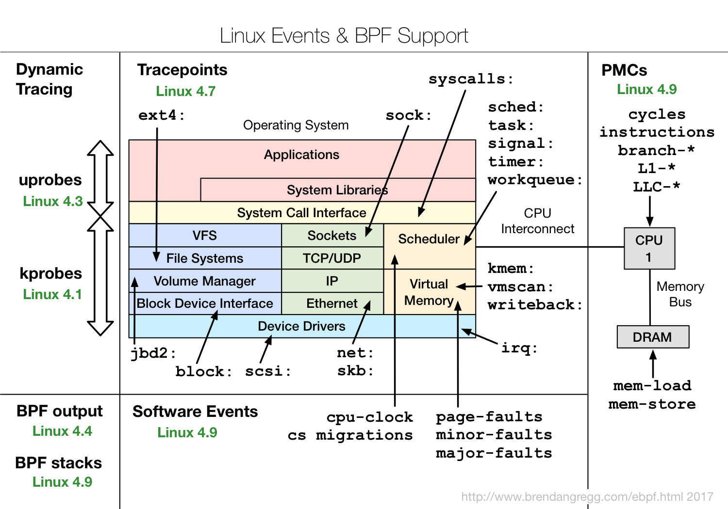
4.1. Prerequisites
A Linux kernel compiled with CONFIG_BPF_SYSCALL (eg, Ubuntu does this), and at least the 4.4 kernel (eg, Ubuntu Xenial) so that histogram, statistic, and per-event tracing is supported. The following diagram shows other features with the Linux version eBPF supported arrived in green:
4.2. Front Ends
There are multiple different front-ends for eBPF. Here's a summary, and I'll cover bcc, bpftrace, and perf in the following sections. I'd recommend trying out bcc and bpftrace (highlighted).
| Front end | Difficulty | Pros | Cons | References |
|---|---|---|---|---|
| BPF bytecode | Brutal | Precise control | Insanely difficult | Kernel source: struct bpf_insn prog in samples/bpf/sock_example.c |
| C | Hard | Build stand-alone binaries | Difficult | Kernel source: samples/bpf/tracex1_kern.c and samples/bpf/tracex1_user.c |
| perf | Hard | Use perf's capabilities: custom events, stack walking | Difficult, not yet well documented | Section below: 7. perf. |
| bcc | Moderate | Custom output, CO-RE binaries, large community, production use (e.g., Facebook, Netflix) | Verbose | Section below: 5. bcc. |
| bpftrace | Easy | Powerful one-liners, many capabilities, growing community, production use (e.g., Netflix, Facebook) | Some limits on code and output | Section below: 6. bpftrace. |
| ply | Easy | Powerful one-liners, small binary, for embedded | Limited control of code and output | github: github.com/iovisor/ply. |
I've previously summarized these on three dimensions: ease of use, scope & capability, and stage of development. Here are the BPF front-ends vs the standard built-in Linux tracers (ftrace and perf):
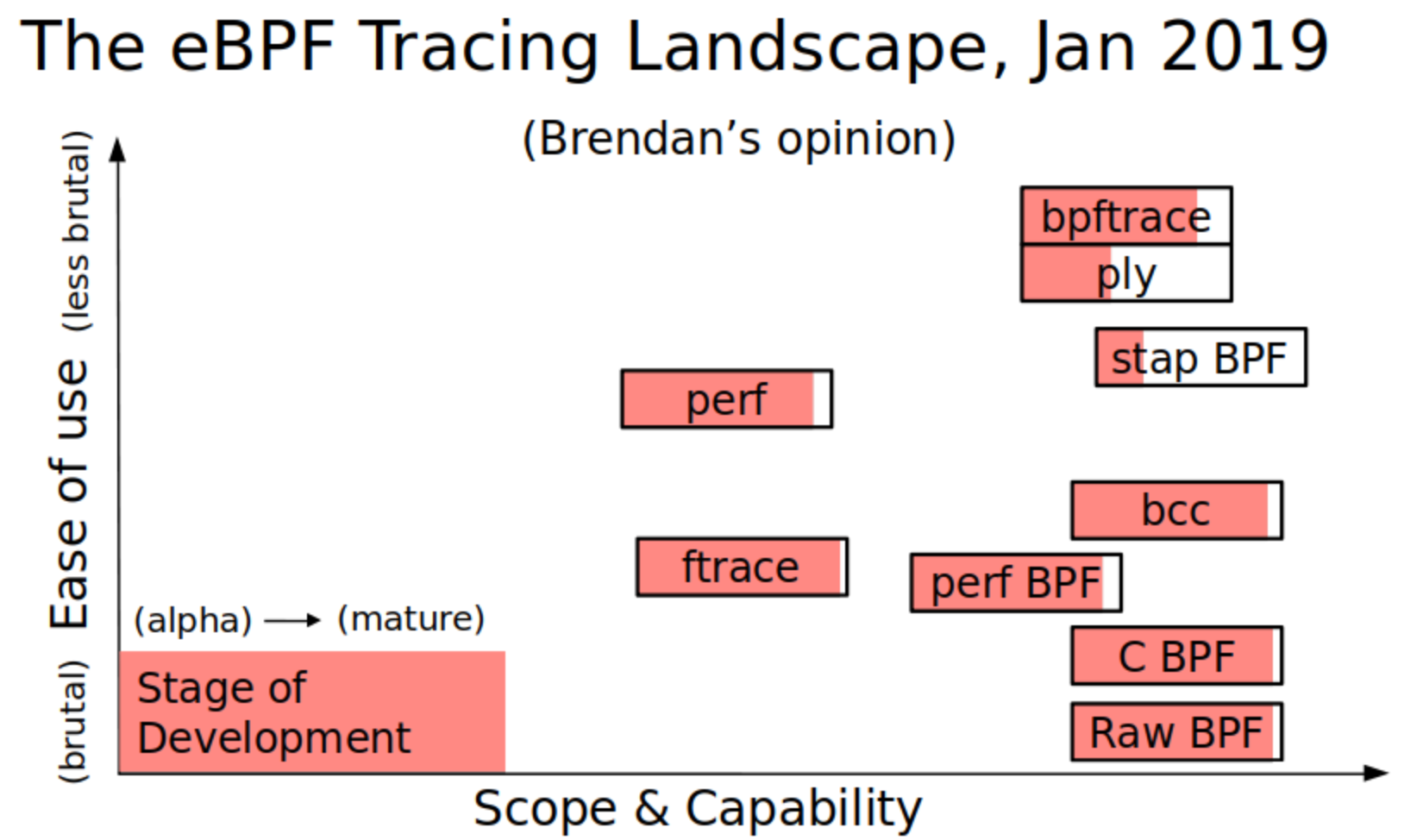
I've shown perf+BPF separately to classic perf and ftrace.
5. BCC
BPF Compiler Collection is on github.com/iovisor/bcc, and provides a large collection of tracing examples tools, as well as C, Python, and lua interfaces for developing them. The diagram on the top right of this page illustrates these bcc tools.
Prerequisites are the same as eBPF above, and Python. If you are on an older kernel (between 4.1 and 4.8) and the bcc tool you want to run doesn't work, take a look in bcc's tools/old directory, which might have a legacy version that employs workarounds.
Example tracing code can be found in the bcc /examples/tracing directory, and in the tools, under the /tools directory. Each tool also has an example .txt file in /tools, and a man page in /man/man8.
I contributed many tools to bcc, including their man pages and examples files, as well as some bcc capabilities and fixes. I also created the tool and events diagrams, the Tutorial, the Developer's Tutorial, the Reference Guide, and published many posts on bcc/eBPF. I'll summarize some content here, but I've written and published a lot more detail in those resources for those wishing to dig deeper.
Update 04-Nov-2020: The Python interface is now considered deprecated in favor of the new C libbpf interface. For more information see my future of BPF perf tools post.
5.1. bcc: Installation
See the bcc install instructions for getting started on different Linux distros. Here are recent Ubuntu instructions, as an example:
# echo "deb [trusted=yes] https://repo.iovisor.org/apt/xenial xenial-nightly main" | \
    sudo tee /etc/apt/sources.list.d/iovisor.list
# sudo apt-get update
# sudo apt-get install bpfcc-tools	# or the old package name: bcc-tools
bcc tools will be installed under /usr/share/bcc/tools.
5.2. bcc: General Performance Checklist
This checklist can be useful if you don't know where to start. It tours various bcc tools to analyze different targets, which may unearth activity you were previously unaware of. I first included this in the bcc tutorial, after a Linux basics checklist of standard tools. It's assumed you've already run such basics (dmesg, vmstat, iostat, top, etc) and now want to dig deeper.
1. execsnoop
Trace new processes via exec() syscalls, and print the parent process name and other details:
# execsnoop
PCOMM            PID    RET ARGS
bash             15887    0 /usr/bin/man ls
preconv          15894    0 /usr/bin/preconv -e UTF-8
man              15896    0 /usr/bin/tbl
man              15897    0 /usr/bin/nroff -mandoc -rLL=169n -rLT=169n -Tutf8
man              15898    0 /usr/bin/pager -s
nroff            15900    0 /usr/bin/locale charmap
nroff            15901    0 /usr/bin/groff -mtty-char -Tutf8 -mandoc -rLL=169n -rLT=169n
groff            15902    0 /usr/bin/troff -mtty-char -mandoc -rLL=169n -rLT=169n -Tutf8
groff            15903    0 /usr/bin/grotty
[...]
2. opensnoop
Trace open() syscalls and print process name and path name details:
# opensnoop
PID    COMM               FD ERR PATH
27159  catalina.sh         3   0 /apps/tomcat8/bin/setclasspath.sh
4057   redis-server        5   0 /proc/4057/stat
2360   redis-server        5   0 /proc/2360/stat
30668  sshd                4   0 /proc/sys/kernel/ngroups_max
30668  sshd                4   0 /etc/group
30668  sshd                4   0 /root/.ssh/authorized_keys
30668  sshd                4   0 /root/.ssh/authorized_keys
30668  sshd               -1   2 /var/run/nologin
30668  sshd               -1   2 /etc/nologin
30668  sshd                4   0 /etc/login.defs
30668  sshd                4   0 /etc/passwd
30668  sshd                4   0 /etc/shadow
30668  sshd                4   0 /etc/localtime
4510   snmp-pass           4   0 /proc/cpuinfo
[...]
3. ext4slower
Trace slow ext4 operations that are slower than a provided threshold (bcc has versions of this for btrfs, XFS, and ZFS as well):
# ext4slower 1
Tracing ext4 operations slower than 1 ms
TIME     COMM           PID    T BYTES   OFF_KB   LAT(ms) FILENAME
06:49:17 bash           3616   R 128     0           7.75 cksum
06:49:17 cksum          3616   R 39552   0           1.34 [
06:49:17 cksum          3616   R 96      0           5.36 2to3-2.7
06:49:17 cksum          3616   R 96      0          14.94 2to3-3.4
06:49:17 cksum          3616   R 10320   0           6.82 411toppm
06:49:17 cksum          3616   R 65536   0           4.01 a2p
06:49:17 cksum          3616   R 55400   0           8.77 ab
06:49:17 cksum          3616   R 36792   0          16.34 aclocal-1.14
06:49:17 cksum          3616   R 15008   0          19.31 acpi_listen
06:49:17 cksum          3616   R 6123    0          17.23 add-apt-repository
06:49:17 cksum          3616   R 6280    0          18.40 addpart
06:49:17 cksum          3616   R 27696   0           2.16 addr2line
06:49:17 cksum          3616   R 58080   0          10.11 ag
4. biolatency
Summarize block device I/O latency as a histogram every second:
# biolatency -mT 1
Tracing block device I/O... Hit Ctrl-C to end.

21:33:40
     msecs               : count     distribution
         0 -> 1          : 69       |****************************************|
         2 -> 3          : 16       |*********                               |
         4 -> 7          : 6        |***                                     |
         8 -> 15         : 21       |************                            |
        16 -> 31         : 16       |*********                               |
        32 -> 63         : 5        |**                                      |
        64 -> 127        : 1        |                                        |

21:33:41
     msecs               : count     distribution
         0 -> 1          : 60       |************************                |
         2 -> 3          : 100      |****************************************|
         4 -> 7          : 41       |****************                        |
         8 -> 15         : 11       |****                                    |
        16 -> 31         : 9        |***                                     |
        32 -> 63         : 6        |**                                      |
        64 -> 127        : 4        |*                                       |

21:33:42
     msecs               : count     distribution
         0 -> 1          : 110      |****************************************|
         2 -> 3          : 78       |****************************            |
         4 -> 7          : 64       |***********************                 |
         8 -> 15         : 8        |**                                      |
        16 -> 31         : 12       |****                                    |
        32 -> 63         : 15       |*****                                   |
        64 -> 127        : 8        |**                                      |
[...]
5. biosnoop
Trace block device I/O with process, disk, and latency details:
# biosnoop
TIME(s)        COMM           PID    DISK    T  SECTOR    BYTES   LAT(ms)
0.000004001    supervise      1950   xvda1   W  13092560  4096       0.74
0.000178002    supervise      1950   xvda1   W  13092432  4096       0.61
0.001469001    supervise      1956   xvda1   W  13092440  4096       1.24
0.001588002    supervise      1956   xvda1   W  13115128  4096       1.09
1.022346001    supervise      1950   xvda1   W  13115272  4096       0.98
1.022568002    supervise      1950   xvda1   W  13188496  4096       0.93
1.023534000    supervise      1956   xvda1   W  13188520  4096       0.79
1.023585003    supervise      1956   xvda1   W  13189512  4096       0.60
2.003920000    xfsaild/md0    456    xvdc    W  62901512  8192       0.23
2.003931001    xfsaild/md0    456    xvdb    W  62901513  512        0.25
2.004034001    xfsaild/md0    456    xvdb    W  62901520  8192       0.35
2.004042000    xfsaild/md0    456    xvdb    W  63542016  4096       0.36
2.004204001    kworker/0:3    26040  xvdb    W  41950344  65536      0.34
2.044352002    supervise      1950   xvda1   W  13192672  4096       0.65
[...]
6. cachestat
Show the page cache hit/miss ratio and size, and summarize every second:
# cachestat
    HITS   MISSES  DIRTIES  READ_HIT% WRITE_HIT%   BUFFERS_MB  CACHED_MB
  170610    41607       33      80.4%      19.6%           11        288
  157693     6149       33      96.2%       3.7%           11        311
  174483    20166       26      89.6%      10.4%           12        389
  434778       35       40     100.0%       0.0%           12        389
  435723       28       36     100.0%       0.0%           12        389
  846183    83800   332534      55.2%       4.5%           13        553
   96387       21       24     100.0%       0.0%           13        553
  120258       29       44      99.9%       0.0%           13        553
  255861       24       33     100.0%       0.0%           13        553
  191388       22       32     100.0%       0.0%           13        553
[...]
7. tcpconnect
Trace TCP active connections (connect()):
# tcpconnect
PID    COMM         IP SADDR            DADDR            DPORT
25333  recordProgra 4  127.0.0.1        127.0.0.1        28527
25338  curl         4  100.66.3.172     52.22.109.254    80
25340  curl         4  100.66.3.172     31.13.73.36      80
25342  curl         4  100.66.3.172     104.20.25.153    80
25344  curl         4  100.66.3.172     50.56.53.173     80
25365  recordProgra 4  127.0.0.1        127.0.0.1        28527
26119  ssh          6  ::1              ::1              22
25388  recordProgra 4  127.0.0.1        127.0.0.1        28527
25220  ssh          6  fe80::8a3:9dff:fed5:6b19 fe80::8a3:9dff:fed5:6b19 22
[...]
8. tcpaccept
Trace TCP passive connections (accept()):
# tcpaccept
PID    COMM         IP RADDR            LADDR            LPORT
2287   sshd         4  11.16.213.254    100.66.3.172     22
4057   redis-server 4  127.0.0.1        127.0.0.1        28527
4057   redis-server 4  127.0.0.1        127.0.0.1        28527
4057   redis-server 4  127.0.0.1        127.0.0.1        28527
4057   redis-server 4  127.0.0.1        127.0.0.1        28527
2287   sshd         6  ::1              ::1              22
4057   redis-server 4  127.0.0.1        127.0.0.1        28527
4057   redis-server 4  127.0.0.1        127.0.0.1        28527
2287   sshd         6  fe80::8a3:9dff:fed5:6b19 fe80::8a3:9dff:fed5:6b19 22
4057   redis-server 4  127.0.0.1        127.0.0.1        28527
[...]
9. tcpretrans
Trace TCP retransmits and TLPs:
# tcpretrans
TIME     PID    IP LADDR:LPORT          T> RADDR:RPORT          STATE
01:55:05 0      4  10.153.223.157:22    R> 69.53.245.40:34619   ESTABLISHED
01:55:05 0      4  10.153.223.157:22    R> 69.53.245.40:34619   ESTABLISHED
01:55:17 0      4  10.153.223.157:22    R> 69.53.245.40:22957   ESTABLISHED
[...]
10. gethostlatency
Show latency for getaddrinfo/gethostbyname[2] library calls, system wide:
# gethostlatency
TIME      PID    COMM          LATms HOST
06:10:24  28011  wget          90.00 www.iovisor.org
06:10:28  28127  wget           0.00 www.iovisor.org
06:10:41  28404  wget           9.00 www.netflix.com
06:10:48  28544  curl          35.00 www.netflix.com.au
06:11:10  29054  curl          31.00 www.plumgrid.com
06:11:16  29195  curl           3.00 www.facebook.com
06:11:24  25313  wget           3.00 www.usenix.org
06:11:25  29404  curl          72.00 foo
06:11:28  29475  curl           1.00 foo
[...]
11. runqlat
Show run queue (scheduler) latency as a histogram, every 5 seconds:
# runqlat -m 5
Tracing run queue latency... Hit Ctrl-C to end.

     msecs               : count     distribution
         0 -> 1          : 2085     |****************************************|
         2 -> 3          : 8        |                                        |
         4 -> 7          : 20       |                                        |
         8 -> 15         : 191      |***                                     |
        16 -> 31         : 420      |********                                |

     msecs               : count     distribution
         0 -> 1          : 1798     |****************************************|
         2 -> 3          : 11       |                                        |
         4 -> 7          : 45       |*                                       |
         8 -> 15         : 441      |*********                               |
        16 -> 31         : 1030     |**********************                  |

     msecs               : count     distribution
         0 -> 1          : 1588     |****************************************|
         2 -> 3          : 7        |                                        |
         4 -> 7          : 49       |*                                       |
         8 -> 15         : 556      |**************                          |
        16 -> 31         : 1206     |******************************          |

[...]
12. profile
Sample stack traces at 49 Hertz, then print unique stacks with the number of occurrences seen:
# profile
Sampling at 49 Hertz of all threads by user + kernel stack... Hit Ctrl-C to end.
^C
[...]
    ffffffff811a2eb0 find_get_entry
    ffffffff811a338d pagecache_get_page
    ffffffff811a51fa generic_file_read_iter
    ffffffff81231f30 __vfs_read
    ffffffff81233063 vfs_read
    ffffffff81234565 SyS_read
    ffffffff818739bb entry_SYSCALL_64_fastpath
    00007f4757ff9680 read
    -                dd (14283)
        29

    ffffffff8141c067 copy_page_to_iter
    ffffffff811a54e8 generic_file_read_iter
    ffffffff81231f30 __vfs_read
    ffffffff81233063 vfs_read
    ffffffff81234565 SyS_read
    ffffffff818739bb entry_SYSCALL_64_fastpath
    00007f407617d680 read
    -                dd (14288)
        32

    ffffffff813af58c common_file_perm
    ffffffff813af6f8 apparmor_file_permission
    ffffffff8136f89b security_file_permission
    ffffffff81232f6e rw_verify_area
    ffffffff8123303e vfs_read
    ffffffff81234565 SyS_read
    ffffffff818739bb entry_SYSCALL_64_fastpath
    00007f407617d680 read
    -                dd (14288)
        39

[...]
5.3. bcc: Tools

The bcc tools section on github lists these with short descriptions. These tools are mostly for performance observability and debugging.
There are two types of tools:
- Single purpose: These tools do one thing and do it well (Unix philosophy). They include execsnoop, opensnoop, ext4slower, biolatency, tcpconnect, oomkill, runqlat, etc. They should be easy to learn and use. Most of the previous examples in the General Performance Checklist were single purpose.
- Multi-tools: These are powerful tools that can do many things, provided you know which arguments and options to use. They featured in the one-liners section earlier on this page, and include trace, argdist, funccount, funclatency, and stackcount.
Each tool has three related parts. Using biolatency as an example:
1/3. The source
$ more libbpf-tools/biolatency.c // SPDX-License-Identifier: (LGPL-2.1 OR BSD-2-Clause) // Copyright (c) 2020 Wenbo Zhang // // Based on biolatency(8) from BCC by Brendan Gregg. // 15-Jun-2020 Wenbo Zhang Created this. #include#include #include #include #include #include #include #include #include "blk_types.h" #include "biolatency.h" #include "biolatency.skel.h" #include "trace_helpers.h" #define ARRAY_SIZE(x) (sizeof(x) / sizeof(*(x))) static struct env { char *disk; time_t interval; int times; [...]
This is the user-space component; in libbpf-tools there is also a biolatency.h header file and a biolatency.bpf.c for kernel BPF code.
Note that bcc also includes the older deprecated versions in Python; E.g.:
$ more tools/biolatency.py
#!/usr/bin/python
# @lint-avoid-python-3-compatibility-imports
#
# biolatency    Summarize block device I/O latency as a histogram.
#               For Linux, uses BCC, eBPF.
#
# USAGE: biolatency [-h] [-T] [-Q] [-m] [-D] [interval] [count]
#
# Copyright (c) 2015 Brendan Gregg.
# Licensed under the Apache License, Version 2.0 (the "License")
#
# 20-Sep-2015   Brendan Gregg   Created this.
[...]
Tools should begin with a block comment to describe basics: what the tool does, its synopsis, major change history.
2/3. An examples file
$ more tools/biolatency_example.txt
Demonstrations of biolatency, the Linux eBPF/bcc version.


biolatency traces block device I/O (disk I/O), and records the distribution
of I/O latency (time), printing this as a histogram when Ctrl-C is hit.
For example:

# ./biolatency
Tracing block device I/O... Hit Ctrl-C to end.
^C
     usecs           : count     distribution
       0 -> 1        : 0        |                                      |
       2 -> 3        : 0        |                                      |
       4 -> 7        : 0        |                                      |
       8 -> 15       : 0        |                                      |
      16 -> 31       : 0        |                                      |
      32 -> 63       : 0        |                                      |
      64 -> 127      : 1        |                                      |
     128 -> 255      : 12       |********                              |
     256 -> 511      : 15       |**********                            |
     512 -> 1023     : 43       |*******************************       |
    1024 -> 2047     : 52       |**************************************|
    2048 -> 4095     : 47       |**********************************    |
    4096 -> 8191     : 52       |**************************************|
    8192 -> 16383    : 36       |**************************            |
   16384 -> 32767    : 15       |**********                            |
   32768 -> 65535    : 2        |*                                     |
   65536 -> 131071   : 2        |*                                     |

The latency of the disk I/O is measured from the issue to the device to its
completion. A -Q option can be used to include time queued in the kernel.

This example output shows a large mode of latency from about 128 microseconds
to about 32767 microseconds (33 milliseconds). The bulk of the I/O was
between 1 and 8 ms, which is the expected block device latency for
rotational storage devices.

The highest latency seen while tracing was between 65 and 131 milliseconds:
the last row printed, for which there were 2 I/O.
[...]
There are detailed examples files in the /tools directory, which include tool output and discussion of what it means.
3/3. A man page
$ nroff -man man/man8/biolatency.8 | more
biolatency(8)                                                    biolatency(8)


NAME
       biolatency - Summarize block device I/O latency as a histogram.

SYNOPSIS
       biolatency [-h] [-T] [-Q] [-m] [-D] [interval [count]]

DESCRIPTION
       biolatency  traces block device I/O (disk I/O), and records the distri-
       bution of I/O latency (time). This is printed as a histogram either  on
       Ctrl-C, or after a given interval in seconds.

       The latency of the disk I/O is measured from the issue to the device to
       its completion. A -Q option can be used to include time queued  in  the
       kernel.

       This  tool uses in-kernel eBPF maps for storing timestamps and the his-
       togram, for efficiency.

       This works by tracing various kernel blk_*()  functions  using  dynamic
       tracing,  and  will  need  updating to match any changes to these func-
       tions.

       Since this uses BPF, only the root user can use this tool.

REQUIREMENTS
       CONFIG_BPF and bcc.

OPTIONS
       -h Print usage message.

       -T     Include timestamps on output.
[...]
The man pages are the reference for what the tool does, what options it has, what the output means including column definitions, and any caveats including overhead.
5.4. bcc: Programming
5.4.1. bcc: Programming: libbpf C
Under construction.
5.4.2. bcc: Programming: Python
While this is generally deprecated, especially with observability tools that have been moving to libbpf C, you may still find a use case where Python is the best fit. Start with the bcc Python Developer Tutorial. It has over 15 lessons that cover all the functions and caveats you'll likely run into. Also see the bcc Reference Guide, which explains the API for the eBPF C and the bcc Python. I created both of these. My goal was to be practical and terse: show real examples and code snippets, cover internals and caveats, and do so as briefly as possible. If you hit page down once or twice, you'll hit the next heading, as I've deliberately kept sections short to avoid a wall of text.
For people who have more of a casual interest in how bcc/BPF is programmed, I'll summarize key things to know next, and then explain the code from one tool in detail.
5 Things To Know
If you want to dive into coding without reading those references, here's five things to know:
- eBPF C is restricted: no unbounded loops or kernel function calls. You can only use the bpf_* functions (and some compiler built-ins).
- All memory must be read onto the BPF stack first before manipulation via bpf_probe_read(), which does necessary checks. If you want to dereference a->b->c->d, then just try doing it first, as bcc has a rewriter that may turn it into the necessary bpf_probe_read()s. If it doesn't work, add explicit bpf_probe_reads()s.
- There are 3 ways to output data from kernel to user:
- bpf_trace_printk(). Debugging only, this writes to trace_pipe and can clash with other programs and tracers. It's very simple, so I've used it early on in the tutorial, but you should use the following instead:
- BPF_PERF_OUTPUT(). A way to sending per-event details to user space, via a custom struct you define. (The Python program currently needs a ct version of the struct definition – this should be automatic one day.)
- BPF_HISTOGRAM() or other BPF maps. Maps are a key-value hash from which more advanced data structures can be built. They can be used for summary statistics or histograms, and read periodically from user space (efficient).
- Use static tracepoints (tracepoints/USDT) instead of dynamic tracing (kprobes/uprobes) wherever possible. It's often not possible, but do try. Dynamic tracing is an unstable API, so your programs will break if the code it's instrumenting changes from one release to another.
- Check for bcc developments or switch to bpftrace. Compared to bpftrace, bcc Python is far more verbose and laborious to code.
Tool example: biolatency.py
The following are all the lines from my original biolatency.py tool, enumerated and commented:
     1	#!/usr/bin/python
     2	# @lint-avoid-python-3-compatibility-imports
Line 1: we're Python. Line 2: I believe suppress a lint warning (these were added for another major companies' build environment).
     3	#
     4	# biolatency    Summarize block device I/O latency as a histogram.
     5	#               For Linux, uses BCC, eBPF.
     6	#
     7	# USAGE: biolatency [-h] [-T] [-Q] [-m] [-D] [interval] [count]
     8	#
     9	# Copyright (c) 2015 Brendan Gregg.
    10	# Licensed under the Apache License, Version 2.0 (the "License")
    11	#
    12	# 20-Sep-2015   Brendan Gregg   Created this.
I have a certain style to my header comments. Line 4 names the tool, and hase a single sentence description. Line 5 adds any caveats: for Linux only, uses BCC/eBPF. It then has a synopsis line, copyright, and a history of major changes.
    13
    14	from __future__ import print_function
    15	from bcc import BPF
    16	from time import sleep, strftime
    17	import argparse
Note that we import BPF, which we'll use to interact with eBPF in the kernel.
    18
    19	# arguments
    20	examples = """examples:
    21	    ./biolatency            # summarize block I/O latency as a histogram
    22	    ./biolatency 1 10       # print 1 second summaries, 10 times
    23	    ./biolatency -mT 1      # 1s summaries, milliseconds, and timestamps
    24	    ./biolatency -Q         # include OS queued time in I/O time
    25	    ./biolatency -D         # show each disk device separately
    26	"""
    27	parser = argparse.ArgumentParser(
    28	    description="Summarize block device I/O latency as a histogram",
    29	    formatter_class=argparse.RawDescriptionHelpFormatter,
    30	    epilog=examples)
    31	parser.add_argument("-T", "--timestamp", action="store_true",
    32	    help="include timestamp on output")
    33	parser.add_argument("-Q", "--queued", action="store_true",
    34	    help="include OS queued time in I/O time")
    35	parser.add_argument("-m", "--milliseconds", action="store_true",
    36	    help="millisecond histogram")
    37	parser.add_argument("-D", "--disks", action="store_true",
    38	    help="print a histogram per disk device")
    39	parser.add_argument("interval", nargs="?", default=99999999,
    40	    help="output interval, in seconds")
    41	parser.add_argument("count", nargs="?", default=99999999,
    42	    help="number of outputs")
    43	args = parser.parse_args()
    44	countdown = int(args.count)
    45	debug = 0
    46
Lines 19 to 44 are argument processing. I'm using Python's argparse here.
My intent is to make this a Unix-like tool, something similar to vmstat/iostat, to make it easy for others to recognize and learn. Hence the style of options and arguments, and also to do one thing and do it well. In this case, showing disk I/O latency as a histogram. I could have added a mode to dump per-event details, but made that a separate tool, biosnoop.py.
You may be writing bcc/eBPF for other reasons, including agents to other monitoring software, and don't need to worry about the user interface.
    47	# define BPF program
    48	bpf_text = """
    49	#include <uapi/linux/ptrace.h>>
    50	#include <linux/blkdev.h>
    51
    52	typedef struct disk_key {
    53	    char disk[DISK_NAME_LEN];
    54	    u64 slot;
    55	} disk_key_t;
    56	BPF_HASH(start, struct request *);
    57	STORAGE
    58
    59	// time block I/O
    60	int trace_req_start(struct pt_regs *ctx, struct request *req)
    61	{
    62	    u64 ts = bpf_ktime_get_ns();
    63	    start.update(&req, &ts);
    64	    return 0;
    65	}
    66
    67	// output
    68	int trace_req_completion(struct pt_regs *ctx, struct request *req)
    69	{
    70	    u64 *tsp, delta;
    71
    72	    // fetch timestamp and calculate delta
    73	    tsp = start.lookup(&req);
    74	    if (tsp == 0) {
    75	        return 0;   // missed issue
    76	    }
    77	    delta = bpf_ktime_get_ns() - *tsp;
    78	    FACTOR
    79
    80	    // store as histogram
    81	    STORE
    82
    83	    start.delete(&req);
    84	    return 0;
    85	}
    86	"""
The eBPF program is declared as an inline C assigned to the variable bpf_text.
Line 56 declares a hash array caled "start", which uses a struct request pointer as the key. The trace_req_start() function fetches a timestamp using bpf_ktime_get_ns() and then stores it in this hash, keyed by *req (I'm just using that pointer address as a UUID). The trace_req_completion() function then does a lookup on the hash with its *req, to fetch the start time of the request, which is then used to calculate the delta time on line 77. Line 83 deletes the timestamp from the hash.
The prototypes to these functions begin with a struct pt_regs * for registers, and then as many of the probed function arguments as you want to include. I've included the first function argument in each, struct request *.
This program also declares storage for the output data and stores it, but there's a problem: biolatency has a -D option to emit per-disk histograms, instead of one histogram for everything, and this changes the storage code. So this eBPF program contains the text STORAGE and STORE (and FACTOR) which are merely strings that we'll search and replace with code next, depending on the options. I'd rather avoid code-that-writes-code if possible, since it makes it harder to debug.
    87
    88	# code substitutions
    89	if args.milliseconds:
    90	    bpf_text = bpf_text.replace('FACTOR', 'delta /= 1000000;')
    91	    label = "msecs"
    92	else:
    93	    bpf_text = bpf_text.replace('FACTOR', 'delta /= 1000;')
    94	    label = "usecs"
    95	if args.disks:
    96	    bpf_text = bpf_text.replace('STORAGE',
    97	        'BPF_HISTOGRAM(dist, disk_key_t);')
    98	    bpf_text = bpf_text.replace('STORE',
    99	        'disk_key_t key = {.slot = bpf_log2l(delta)}; ' +
   100	        'bpf_probe_read(&key.disk, sizeof(key.disk), ' +
   101	        'req->rq_disk->disk_name); dist.increment(key);')
   102	else:
   103	    bpf_text = bpf_text.replace('STORAGE', 'BPF_HISTOGRAM(dist);')
   104	    bpf_text = bpf_text.replace('STORE',
   105	        'dist.increment(bpf_log2l(delta));')
The FACTOR code just changes the units of the time we're recording, depending on the -m option.
Line 95 checks if per-disk has been requested (-D), and if so, replaces the STORAGE and STORE strings with code to do per-disk histograms. It uses the disk_key struct declared on line 52 which is the disk name and the slot (bucket) in the power-of-2 histogram. Line 99 takes the delta time and turns it into the power-of-2 slot index using the bpf_log2l() helper function. Lines 100 and 101 fetch the disk name via bpf_probe_read(), which is how all data is copied onto BPF's stack for operation. Line 101 includes many dereferences: req->rq_disk, rq_disk->disk_name: bcc's rewriter has transparently turned these into bpf_probe_read()s as well.
Lines 103 to 105 deal with the single histogram case (not per-disk). A histogram is declared named "dist" using the BPF_HISTOGRAM macro. The slot (bucket) is found using the bpf_log2l() helper function, and then incremented in the histogram.
This example is a little gritty, which is both good (realistic) and bad (intimidating). See the tutorial I linked to earlier for more simple examples.
   106	if debug:
   107	    print(bpf_text)
Since I have code that writes code, I need a way to debug the final output. If debug is set, print it out.
   108
   109	# load BPF program
   110	b = BPF(text=bpf_text)
   111	if args.queued:
   112	    b.attach_kprobe(event="blk_account_io_start", fn_name="trace_req_start")
   113	else:
   114	    b.attach_kprobe(event="blk_start_request", fn_name="trace_req_start")
   115	    b.attach_kprobe(event="blk_mq_start_request", fn_name="trace_req_start")
   116	b.attach_kprobe(event="blk_account_io_completion",
   117	    fn_name="trace_req_completion")
   118
Line 110 loads the eBPF program.
Since this program was written before eBPF had tracepoint support, I wrote it to use kprobes (kernel dynamic tracing). It should be rewritten to use tracepoints, as they are a stable API, although that then also requires a later kernel version (Linux 4.7+).
biolatency.py has a -Q option to included time queued in the kernel. We can see how it's implemented in this code. If it is set, line 112 attaches our eBPF trace_req_start() function with a kprobe on the blk_account_io_start() kernel function, which tracks the request when it's first queued in the kernel. If not set, lnes 114 and 115 attach our eBPF function to different kernel functions, which is when the disk I/O is issued (it can be either of these). This only works because the first argument to any of these kernels functions is the same: struct request *. If their arguments were different, I'd need separate eBPF functions for each to handle that.
   119	print("Tracing block device I/O... Hit Ctrl-C to end.")
   120
   121	# output
   122	exiting = 0 if args.interval else 1
   123	dist = b.get_table("dist")
Line 123 fetches the "dist" histogram that was declared and populated by the STORAGE/STORE code.
   124	while (1):
   125	    try:
   126	        sleep(int(args.interval))
   127	    except KeyboardInterrupt:
   128	        exiting = 1
   129
   130	    print()
   131	    if args.timestamp:
   132	        print("%-8s\n" % strftime("%H:%M:%S"), end="")
   133
   134	    dist.print_log2_hist(label, "disk")
   135	    dist.clear()
   136
   137	    countdown -= 1
   138	    if exiting or countdown == 0:
   139	        exit()
This has logic for printing every interval, a certain number of times (countdown). Lines 131 and 132 print a timestamp if the -T option was used.
Line 134 prints the histogram, or histograms if we're doing per-disk. The first argument is the label variable, which contains "usecs" or "msecs", and decorates the column of values in the output. The second argument is labels the secondary key, if dist has per-disk histograms. How print_log2_hist() can identify whether this is a single histogram or has a secondary key, I'll leave as an adventurous exercise in code spelunking of bcc and eBPF internals.
Line 135 clears the histogram, ready for the next interval.
Here is some sample output:
# biolatency
Tracing block device I/O... Hit Ctrl-C to end.
^C
     usecs           : count     distribution
       0 -> 1        : 0        |                                      |
       2 -> 3        : 0        |                                      |
       4 -> 7        : 0        |                                      |
       8 -> 15       : 0        |                                      |
      16 -> 31       : 0        |                                      |
      32 -> 63       : 0        |                                      |
      64 -> 127      : 1        |                                      |
     128 -> 255      : 12       |********                              |
     256 -> 511      : 15       |**********                            |
     512 -> 1023     : 43       |*******************************       |
    1024 -> 2047     : 52       |**************************************|
    2048 -> 4095     : 47       |**********************************    |
    4096 -> 8191     : 52       |**************************************|
    8192 -> 16383    : 36       |**************************            |
   16384 -> 32767    : 15       |**********                            |
   32768 -> 65535    : 2        |*                                     |
   65536 -> 131071   : 2        |*                                     |
Per-disk output:
# biolatency -D
Tracing block device I/O... Hit Ctrl-C to end.
^C
disk = 'xvdb'
     usecs               : count     distribution
         0 -> 1          : 0        |                                        |
         2 -> 3          : 0        |                                        |
         4 -> 7          : 0        |                                        |
         8 -> 15         : 0        |                                        |
        16 -> 31         : 0        |                                        |
        32 -> 63         : 0        |                                        |
        64 -> 127        : 18       |****                                    |
       128 -> 255        : 167      |****************************************|
       256 -> 511        : 90       |*********************                   |

disk = 'xvdc'
     usecs               : count     distribution
         0 -> 1          : 0        |                                        |
         2 -> 3          : 0        |                                        |
         4 -> 7          : 0        |                                        |
         8 -> 15         : 0        |                                        |
        16 -> 31         : 0        |                                        |
        32 -> 63         : 0        |                                        |
        64 -> 127        : 22       |****                                    |
       128 -> 255        : 179      |****************************************|
       256 -> 511        : 88       |*******************                     |

disk = 'xvda1'
     usecs               : count     distribution
         0 -> 1          : 0        |                                        |
         2 -> 3          : 0        |                                        |
         4 -> 7          : 0        |                                        |
         8 -> 15         : 0        |                                        |
        16 -> 31         : 0        |                                        |
        32 -> 63         : 0        |                                        |
        64 -> 127        : 0        |                                        |
       128 -> 255        : 0        |                                        |
       256 -> 511        : 167      |****************************************|
       512 -> 1023       : 44       |**********                              |
      1024 -> 2047       : 9        |**                                      |
      2048 -> 4095       : 4        |                                        |
      4096 -> 8191       : 34       |********                                |
      8192 -> 16383      : 44       |**********                              |
     16384 -> 32767      : 33       |*******                                 |
     32768 -> 65535      : 1        |                                        |
     65536 -> 131071     : 1        |                                        |
From the output we can see that xvdb and xvdc have similar latency histograms, whereas xvda1 is quite different and bimodal, with a higher latency mode between 4 and 32 milliseconds.
6. bpftrace
bpftrace is at github.com/iovisor/bpftrace, and is a high-level front-end for BPF tracing, which uses libraries from bcc. bpftrace is ideal for ad hoc instrumentation with powerful custom one-liners and short scripts, whereas bcc is ideal for complex tools and daemons. bpftrace was created by Alastair Robertson as a spare time project.
I contributed many capabilities and fixes to bpftrace, as well as tools and their example files and man pages. I also created the bpftrace One-Liners Tutorial, the Reference Guide, and the Internals Development Guide, and published blog posts. I'll summarize bpftrace here, but I've written and published a lot more detail in those resources for those wishing to dig deeper.
6.1. bpftrace: Installation
See the bpftrace install instructions for getting started on different Linux distros. One of these might be possible!:
# snap install bpftrace
# yum install bpftrace
# apt-get install bpftrace
But these are still under development, and you may need to refer to the full instructions in the previous link to get it to work. The only place I know where it "just works" is within some large tech companies who have built it in their internal repos.
To test if your install works, try a basic one-liner:
# sudo bpftrace -e 'BEGIN { printf("Hello BPF!\n"); exit(); }'
Attaching 1 probe...
Hello BPF!
6.2. bpftrace: One-Liners
The following are from my One-Liners Tutorial, which has more details on each:
1. Listing probes
bpftrace -l 'tracepoint:syscalls:sys_enter_*'

2. Hello world
bpftrace -e 'BEGIN { printf("hello world\n"); }'

3. File opens
bpftrace -e 'tracepoint:syscalls:sys_enter_open { printf("%s %s\n", comm, str(args->filename)); }'

4. Syscall counts by process
bpftrace -e 'tracepoint:raw_syscalls:sys_enter { @[comm] = count(); }'

5. Distribution of read() bytes
bpftrace -e 'tracepoint:syscalls:sys_exit_read /pid == 18644/ { @bytes = hist(args->retval); }'

6. Kernel dynamic tracing of read() bytes
bpftrace -e 'kretprobe:vfs_read { @bytes = lhist(retval, 0, 2000, 200); }'

7. Timing read()s
bpftrace -e 'kprobe:vfs_read { @start[tid] = nsecs; }
    kretprobe:vfs_read /@start[tid]/ { @ns[comm] = hist(nsecs - @start[tid]); delete(@start[tid]); }'

8. Count process-level events
bpftrace -e 'tracepoint:sched:sched* { @[name] = count(); } interval:s:5 { exit(); }'

9. Profile on-CPU kernel stacks
bpftrace -e 'profile:hz:99 { @[stack] = count(); }'

10. Scheduler tracing
bpftrace -e 'tracepoint:sched:sched_switch { @[stack] = count(); }'

11. Block I/O tracing
bpftrace -e 'tracepoint:block:block_rq_complete { @ = hist(args->nr_sector * 512); }'
If you can run and understand these one-liners, you'll have learned a lot of bpftrace.
Here is some output of file opens:
# bpftrace -e 'tracepoint:syscalls:sys_enter_open { printf("%s %s\n", comm, str(args->filename)); }'
Attaching 1 probe...
snmpd /proc/net/dev
snmpd /proc/net/if_inet6
snmpd /sys/class/net/docker0/device/vendor
snmpd /proc/sys/net/ipv4/neigh/docker0/retrans_time_ms
snmpd /proc/sys/net/ipv6/neigh/docker0/retrans_time_ms
snmpd /proc/sys/net/ipv6/conf/docker0/forwarding
snmpd /proc/sys/net/ipv6/neigh/docker0/base_reachable_time_ms
snmpd /sys/class/net/eth0/device/vendor
snmpd /sys/class/net/eth0/device/device
snmpd /proc/sys/net/ipv4/neigh/eth0/retrans_time_ms
snmpd /proc/sys/net/ipv6/neigh/eth0/retrans_time_ms
snmpd /proc/sys/net/ipv6/conf/eth0/forwarding
snmpd /proc/sys/net/ipv6/neigh/eth0/base_reachable_time_ms
snmpd /sys/class/net/lo/device/vendor
snmpd /proc/sys/net/ipv4/neigh/lo/retrans_time_ms
snmpd /proc/sys/net/ipv6/neigh/lo/retrans_time_ms
snmpd /proc/sys/net/ipv6/conf/lo/forwarding
snmpd /proc/sys/net/ipv6/neigh/lo/base_reachable_time_ms
snmp-pass /proc/cpuinfo
snmp-pass /proc/stat
Tracing which files have been opened can be a quick way to locate config files, log files, data files, libraries, and other things of interest.
Here is some output of timing read()s:
# bpftrace -e 'kprobe:vfs_read { @start[tid] = nsecs; }
    kretprobe:vfs_read /@start[tid]/ { @ns[comm] = hist(nsecs - @start[tid]); delete(@start[tid]); }'
Attaching 2 probes...
^C

@ns[sleep]:
[1K, 2K)               1 |@@@@@@@@@@@@@@@@@@@@@@@@@@@@@@@@@@@@@@@@@@@@@@@@@@@@|

@ns[ls]:
[256, 512)             1 |@@@@@@@@@@@@@@@@@                                   |
[512, 1K)              3 |@@@@@@@@@@@@@@@@@@@@@@@@@@@@@@@@@@@@@@@@@@@@@@@@@@@@|
[1K, 2K)               1 |@@@@@@@@@@@@@@@@@                                   |
[2K, 4K)               1 |@@@@@@@@@@@@@@@@@                                   |
[4K, 8K)               0 |                                                    |
[8K, 16K)              0 |                                                    |
[16K, 32K)             1 |@@@@@@@@@@@@@@@@@                                   |

@ns[systemd]:
[4K, 8K)               9 |@@@@@@@@@@@@@@@@@@@@@@@@@@@@@@@@@@@@@@@@@@@@@@@@@@@@|

@ns[snmpd]:
[512, 1K)             18 |@@@@@@@@@@@@@@@@@@@@@@@@@@@@@@@@@@@@@@@@@@@@@@@@@@@@|
[1K, 2K)               3 |@@@@@@@@                                            |
[2K, 4K)               9 |@@@@@@@@@@@@@@@@@@@@@@@@@@                          |
[4K, 8K)               2 |@@@@@                                               |
[8K, 16K)              3 |@@@@@@@@                                            |
[16K, 32K)             3 |@@@@@@@@                                            |
[32K, 64K)             1 |@@                                                  |
[64K, 128K)            0 |                                                    |
[128K, 256K)           1 |@@                                                  |

@ns[snmp-pass]:
[256, 512)             6 |@@@@@@@                                             |
[512, 1K)              4 |@@@@                                                |
[1K, 2K)               0 |                                                    |
[2K, 4K)               0 |                                                    |
[4K, 8K)               0 |                                                    |
[8K, 16K)              0 |                                                    |
[16K, 32K)             1 |@                                                   |
[32K, 64K)            13 |@@@@@@@@@@@@@@@                                     |
[64K, 128K)            3 |@@@                                                 |
[128K, 256K)          43 |@@@@@@@@@@@@@@@@@@@@@@@@@@@@@@@@@@@@@@@@@@@@@@@@@@@@|
[256K, 512K)           5 |@@@@@@                                              |

@ns[sshd]:
[1K, 2K)               7 |@@@@@@@@@@                                          |
[2K, 4K)              30 |@@@@@@@@@@@@@@@@@@@@@@@@@@@@@@@@@@@@@@@@@@@@        |
[4K, 8K)              35 |@@@@@@@@@@@@@@@@@@@@@@@@@@@@@@@@@@@@@@@@@@@@@@@@@@@@|
[8K, 16K)             33 |@@@@@@@@@@@@@@@@@@@@@@@@@@@@@@@@@@@@@@@@@@@@@@@@@   |
[16K, 32K)             1 |@                                                   |
The ASCII histogram shows the distribution of the latency, helping you see if it is multi-modal, or if there are latency outliers.
6.3. bpftrace: Programming Summary
This is a summary/cheat sheet for programming in bpftrace. See the bpftrace reference guide for more information.
This is also available as a separate page you can print out: bpftrace cheat sheet.
Syntax
probe[,probe,...] /filter/ { action }
The probe specifies what events to instrument, the filter is optional and can filter down the events based on a boolean expression, and the action is the mini program that runs.
Here's hello world:
# bpftrace -e 'BEGIN { printf("Hello eBPF!\n"); }'
The probe is BEGIN, a special probe that runs at the beginning of the program (like awk). There's no filter. The action is a printf() statement.
Now a real example:
# bpftrace -e 'kretprobe:vfs_read /pid == 181/ { @bytes = hist(retval); }'
This uses a kretprobe to instrument the return of the sys_read() kernel function. If the PID is 181, a special map variable @bytes is populated with a log2 histogram function with the return value retval of sys_read(). This produces a histogram of the returned read size for PID 181. Is your app doing lots of 1 byte reads? Maybe that can be optimized.
Probe Types
These are libraries of probes which are related. The currently supported types are (more will be added):
| Alias | Type | Description |
|---|---|---|
| t | tracepoint | Kernel static instrumentation points |
| U | usdt | User-level statically defined tracing |
| k | kprobe | Kernel dynamic function instrumentation (standard) |
| kr | kretprobe | Kernel dynamic function return instrumentation (standard) |
| f | kfunc | Kernel dynamic function instrumentation (BPF based) |
| fr | kretfunc | Kernel dynamic function return instrumentation (BPF based) |
| u | uprobe | User-level dynamic function instrumentation |
| ur | uretprobe | User-level dynamic function return instrumentation |
| s | software | Kernel software-based events |
| h | hardware | Hardware counter-based instrumentation |
| w | watchpoint | Memory watchpoint events |
| p | profile | Timed sampling across all CPUs |
| i | interval | Timed reporting (from one CPU) |
| iter | Iterator tracing over kernel objects | |
| BEGIN | Start of bpftrace | |
| END | End of bpftrace |
Dynamic instrumentation lets you trace any software function in a running binary without restarting it. However, the functions it exposes are not considered a stable API, as they can change from one software version to another, breaking the bpftrace tools you develop. Try to use the static probe types wherever possible, as they are usually best effort stable.
Variable Types
| Variable | Description |
|---|---|
| @name | global |
| @name[key] | hash |
| @name[tid] | thread-local |
| $name | scratch |
Variables with a '@' prefix use BPF maps, which can behave like associative arrays. They can be populated in one of two ways:
- variable assignment: @name = x;
- function assignment: @name = hist(x);
There are various map-populating functions as builtins that provide quick ways to summarize data.
Builtin Variables
| Variable | Description |
|---|---|
| pid | Process ID |
| tid | Thread ID |
| uid | User ID |
| username | Username |
| comm | Process or command name |
| curtask | Current task_struct as a u64 |
| nsecs | Current time in nanoseconds |
| elapsed | Time in nanoseconds since bpftrace start |
| kstack | Kernel stack trace |
| ustack | User-level stack trace |
| arg0...argN | Function arguments |
| args | Tracepoint arguments |
| retval | Function return value |
| func | Function name |
| probe | Full probe name |
| $1...$N | Positional parameters |
| cgroup | Default cgroup v2 ID |
Builtin Functions
| Function | Description |
|---|---|
| printf("...") | Print formatted string |
| time("...") | Print formatted time |
| join(char *arr[]) | Join array of strings with a space |
| str(char *s [, int length]) | Return string from s pointer |
| buf(void *p [, int length]) | Return a hexadecimal string from p pointer |
| strncmp(char *s1, char *s2, int length) | Compares two strings up to length |
| sizeof(expression) | Returns the size of the expression |
| kstack([limit]) | Kernel stack trace up to limit frames |
| ustack([limit]) | User-level stack trace up to limit frames |
| ksym(void *p) | Resolve kernel address to symbol |
| usym(void *p) | Resolve user-space address to symbol |
| kaddr(char *name) | Resolve kernel symbol name to address |
| uaddr(char *name) | Resolve user-space symbol name to address |
| ntop([int af,]int|char[4:16] addr) | Convert IP address data to text |
| reg(char *name) | Return register value |
| cgroupid(char *path) | Return cgroupid for /sys/fs/cgroup/... path |
| time("...") | Print formatted time |
| system("...") | Run shell command |
| cat(char *filename) | Print file content |
| signal(char[] sig | int sig) | Send a signal to the current task |
| override(u64 rc) | Override a kernel function return value |
| exit() | Exits bpftrace |
| @ = count() | Count events |
| @ = sum(x) | Sum the value |
| @ = hist(x) | Power-of-2 histogram for x |
| @ = lhist(x, min, max, step) | Linear histogram for x |
| @ = min(x) | Record the minimum value seen |
| @ = max(x) | Record the maximum value seen |
| @ = stats(x) | Return the count, average, and total for this value |
| delete(@x[key]) | Delete the map element |
| clear(@x) | Delete all keys from the map |
There are additional lesser-used functions and capabilities not summarized here. See the Reference Guide.
7. perf
eBPF can also be used from the Linux perf command (aka perf_events) in Linux 4.4 and newer. The newer the better, as perf/BPF support keeps improving with each release. I've provided one example so far on my perf page: perf eBPF.
8. References
- bcc (BPF Compiler Collection) (github): tools, tutorial, reference guide, examples, man pages.
- BPF docs (github): BPF docs.
- Documentation/networking/filter.txt (kernel.org) BPF & eBPF docs in the kernel source.
9. Other eBPF Uses
Other uses outside of observability. Just links for now.
- Cilium: API-aware networking and security.
- Yet another new approach to seccomp by Jonathan Corbet.
- eBPF/XDP SmartNIC offload (slides) by David Beckett and Jakub Kicinski (Netronome).
- When eBPF Meets FUSE (PDF) slides for OSS, by Ashish Bijlani.
- Why is the kernel community replacing iptables with BPF? by Thomas Graf (cilium).
10. Acknowledgements
Many people have worked on tracers and contributed in different ways over the years to get to where we are today, including those who worked on the Linux frameworks that bcc/eBPF makes use of: tracepoints, kprobes, uprobes, ftrace, and perf_events. The most recent contributors include Alexei Starovoitov and Daniel Borkmann, who have lead eBPF development, and Brenden Blanco and Yonghong Song, who have lead bcc development. Many of the single purpose bcc tools were written by me (execsnoop, opensnoop, biolatency, ext4slower, tcpconnect, gethostlatency, etc), and two of the most important multi-tools (trace and argdist) were written by Sasha Goldshtein. I wrote a longer list of acknowledgements at the end of this post. Thank you everyone!
11. Updates
Other resources about eBPF for observability, organized by year. (I'm still updating these updates...)
2013
- enhanced BPF by Alexei Starovoitov
- tracing filters with BPF by Alexei Starovoitov
2014
- BPF syscall, maps, verifier, samples by Alexei Starovoitov
2015
2016
- Linux eBPF Stack Trace Hack (bcc)
- Linux eBPF Off-CPU Flame Graph (bcc)
- Linux Wakeup and Off-Wake Profiling (bcc)
- Linux chain graph prototype (bcc)
- Linux 4.x Performance: Using BPF Superpowers (slides)
- Linux eBPF/bcc uprobes
- Linux BPF/bcc Road Ahead
- Ubuntu Xenial bcc/BPF
- Dive into BPF: a list of reading material by Quentin Monnet
- Linux bcc/BPF Tracing Security Capabilities
- Linux MySQL Slow Query Tracing with bcc/BPF
- Linux bcc/BPF ext4 Latency Tracing
- Linux bcc/BPF Run Queue (Scheduler) Latency
- Linux bcc/BPF Node.js USDT Tracing
- Staring into the eBPF Abyss (slides) by Sasha Goldshtein.
- Meet-cute between eBPF and Kernel Tracing (slides) by Viller Hsiao.
- eBPF Trace from Kernel to Userspace (slides) by Gary Lin.
- Linux bcc tcptop
- Linux 4.9's Efficient BPF-based Profiler
- DTrace for Linux 2016
- Linux 4.x Tracing Tools: Using BPF Superpowers (slides)
- Linux bcc/BPF tcplife: TCP Lifespans
2017
- Golang bcc/BPF Function Tracing
- BPF: Tracing and More (slides) (youtube)
- eBPF, part1: Past, Present, and Future by Ferris Ellis
- eBPF, part 2: Syscall and Map Types by Ferris Ellis
- Performance Analysis Superpowers with Linux eBPF (slides) (youtube)
- Optimizing web servers for high throughput and low latency (uses some bcc/BPF) by Alexey Ivanov.
- Linux 4.x Tracing: Performance Analysis with bcc/BPF (slides) (youtube)
- A thorough introduction to eBPF by Matt Fleming.
- 7 tools for analyzing performance in Linux with bcc/BPF.
- JVM Monitoring with BPF at USENIX LISA17.
2018
- BPFd: Running BCC tools remotely across systems and architectures by Joel Fernandes
- KPTI/KAISER Meltdown performance analysis (includes some bcc/BPF analysis)
- Writing eBPF tracing tools in Rust by Julia Evans.
- Prototyping an ltrace clone using eBPF by Julia Evans.
- Some advanced BCC topics by Matt Fleming.
- Using user-space tracepoints with BPF by Matt Fleming.
- Linux system monitoring with eBPF by Circonus.
- TCP Tracepoints
- eBPF maps 101 by Al Cho (SUSE).
- Linux bcc/eBPF tcpdrop Linux System Monitoring with eBPF (slides) by Heinrich Hartmann (Circonus).
- BPF verifier future by Alexei Starovoitov.
- Sysdig developes eBPF support by Gianluca Borello.
- Low-Overhead System Tracing With eBPF (youtube) talk (slides) by Akshay Kapoor.
- Building Network Functions with eBPF & BCC (slides) by Shmulik Ladkani (Meta Networks).
- Taking eBPF (bcc tools) for a quick spin in RHEL 7.6 (beta), by Allan McAleavy.
- Introducing ebpf_exporter by Ivan Babrou (Cloudflare).
- How I ended up writing opensnoop in pure C using eBPF by Michael Bolin.
- High-level tracing with bpftrace by Colin Ian King.
- eBPF Powered Distributed Kubernetes Performance Analysis (video) talk at KubeCon by Lorenzo Fontana.
- Low-Overhead Tracing Using eBPF for Observability into Kubernetes Apps and Services (video) talk at KubeCon by Gaurav Gupta.
- Linux: easy keylogger with eBPF by Andrea Righi.
2019
- From High Ceph Latency to Kernel Patch with eBPF/BCC by Алексей Захаров.
- Learn eBPF Tracing: Tutorial and Examples by myself.
- BPF Performance Tools: Linux System and Application Observability (book) by myself, published by Addison Wesley.
- Kernel analysis with bpftrace (lwn.net) by myself.
- Playing with BPF by Kir Shatrov.
- A thorough introduction to bpftrace by myself.
- BPF: A New Type of Software by myself.
- BPF Theremin, Tetris, and Typewriters by myself.
- BPF binaries: BTF, CO-RE, and the future of BPF perf tools by myself.
2020
- Unlocking eBPF power by Michał Wcisło shows a proof of concept tool that unlocks your laptop when your phone is nearby, using bpftrace.
- ebpf.io: eBPF (BPF) now has its own website.
- BPF binaries: BTF, CO-RE, and the future of BPF perf tools by myself.
2021
- USENIX LISA2021 BPF Internals (eBPF) by myself.
- How To Add eBPF Observability To Your Product by myself.