
Load averages are an industry-critical metric – my company spends millions auto-scaling cloud instances based on them and other metrics – but on Linux there's some mystery around them. Linux load averages track not just runnable tasks, but also tasks in the uninterruptible sleep state. Why? I've never seen an explanation. In this post I'll solve this mystery, and summarize load averages as a reference for everyone trying to interpret them.
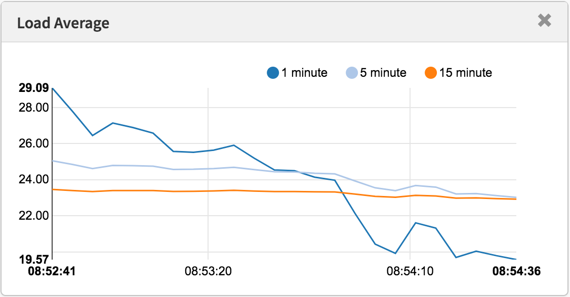
Linux load averages are "system load averages" that show the running thread (task) demand on the system as an average number of running plus waiting threads. This measures demand, which can be greater than what the system is currently processing. Most tools show three averages, for 1, 5, and 15 minutes:
$ uptime
 16:48:24 up  4:11,  1 user,  load average: 25.25, 23.40, 23.46

top - 16:48:42 up  4:12,  1 user,  load average: 25.25, 23.14, 23.37

$ cat /proc/loadavg
25.72 23.19 23.35 42/3411 43603
Some interpretations:
- If the averages are 0.0, then your system is idle.
- If the 1 minute average is higher than the 5 or 15 minute averages, then load is increasing.
- If the 1 minute average is lower than the 5 or 15 minute averages, then load is decreasing.
- If they are higher than your CPU count, then you might have a performance problem (it depends).
As a set of three, you can tell if load is increasing or decreasing, which is useful. They can be also useful when a single value of demand is desired, such as for a cloud auto scaling rule. But to understand them in more detail is difficult without the aid of other metrics. A single value of 23 - 25, by itself, doesn't mean anything, but might mean something if the CPU count is known, and if it's known to be a CPU-bound workload.
Instead of trying to debug load averages, I usually switch to other metrics. I'll discuss these in the "Better Metrics" section near the end.
History
The original load averages show only CPU demand: the number of processes running plus those waiting to run. There's a nice description of this in RFC 546 titled "TENEX Load Averages", August 1973:
[1] The TENEX load average is a measure of CPU demand. The load average is an average of the number of runnable processes over a given time period. For example, an hourly load average of 10 would mean that (for a single CPU system) at any time during that hour one could expect to see 1 process running and 9 others ready to run (i.e., not blocked for I/O) waiting for the CPU.
The version of this on ietf.org links to a PDF scan of a hand drawn load average graph from July 1973, showing that this has been monitored for decades:
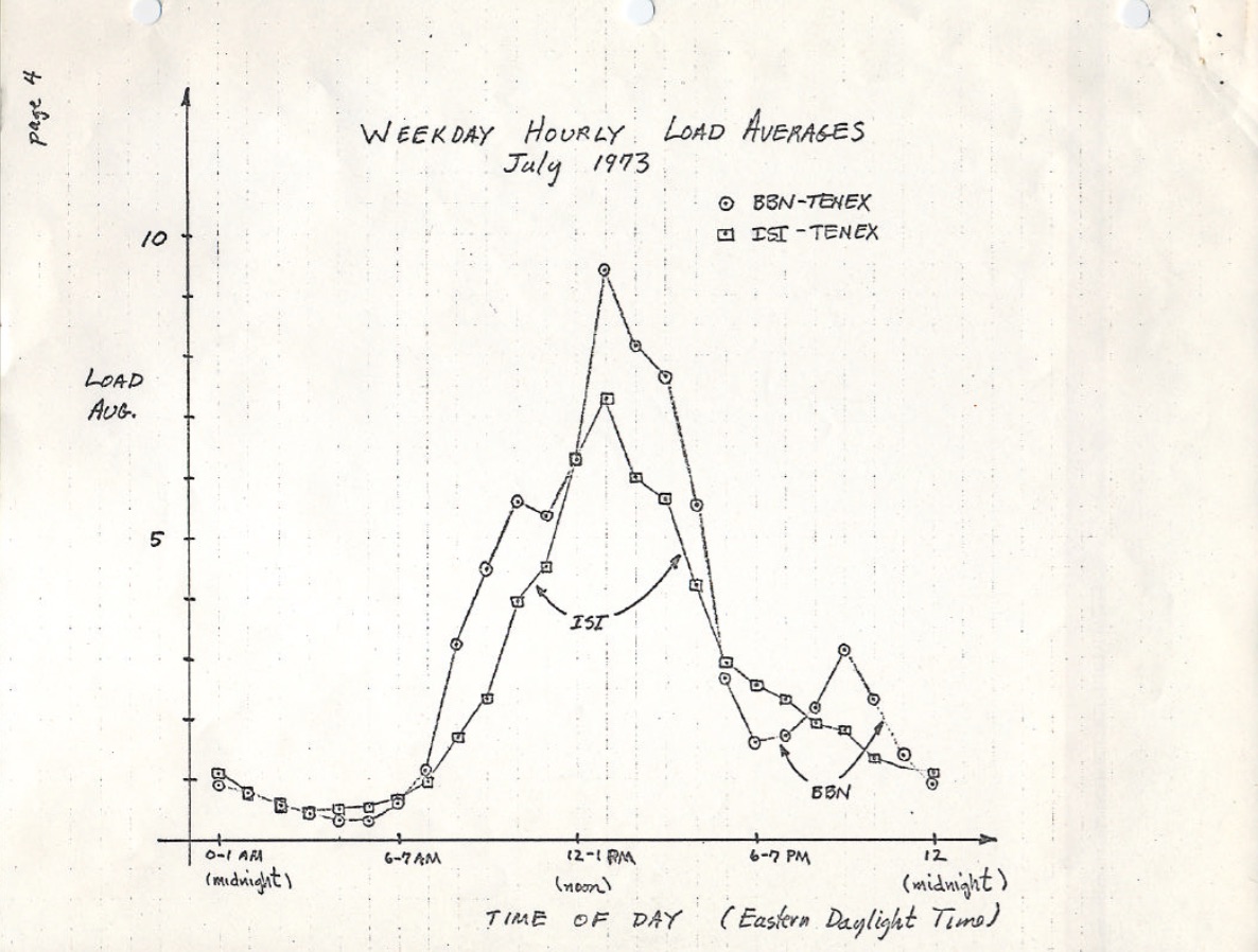
source: https://tools.ietf.org/html/rfc546
Nowadays, the source code to old operating systems can also be found online. Here's an except of DEC macro assembly from TENEX (early 1970's) SCHED.MAC:
NRJAVS==3               ;NUMBER OF LOAD AVERAGES WE MAINTAIN
GS RJAV,NRJAVS          ;EXPONENTIAL AVERAGES OF NUMBER OF ACTIVE PROCESSES
[...]
;UPDATE RUNNABLE JOB AVERAGES

DORJAV: MOVEI 2,^D5000
        MOVEM 2,RJATIM          ;SET TIME OF NEXT UPDATE
        MOVE 4,RJTSUM           ;CURRENT INTEGRAL OF NBPROC+NGPROC
        SUBM 4,RJAVS1           ;DIFFERENCE FROM LAST UPDATE
        EXCH 4,RJAVS1
        FSC 4,233               ;FLOAT IT
        FDVR 4,[5000.0]         ;AVERAGE OVER LAST 5000 MS
[...]
;TABLE OF EXP(-T/C) FOR T = 5 SEC.

EXPFF:  EXP 0.920043902 ;C = 1 MIN
        EXP 0.983471344 ;C = 5 MIN
        EXP 0.994459811 ;C = 15 MIN
And here's an excerpt from Linux today (include/linux/sched/loadavg.h):
#define EXP_1           1884            /* 1/exp(5sec/1min) as fixed-point */
#define EXP_5           2014            /* 1/exp(5sec/5min) */
#define EXP_15          2037            /* 1/exp(5sec/15min) */
Linux is also hard coding the 1, 5, and 15 minute constants.
There have been similar load average metrics in older systems, including Multics, which had an exponential scheduling queue average.
The Three Numbers
These three numbers are the 1, 5, and 15 minute load averages. Except they aren't really averages, and they aren't 1, 5, and 15 minutes. As can be seen in the source above, 1, 5, and 15 minutes are constants used in an equation, which calculate exponentially-damped moving sums of a five second average. The resulting 1, 5, and 15 minute load averages reflect load well beyond 1, 5, and 15 minutes.
If you take an idle system, then begin a single-threaded CPU-bound workload (one thread in a loop), what would the one minute load average be after 60 seconds? If it was a plain average, it would be 1.0. Here is that experiment, graphed:

Load average experiment to visualize exponential damping
The so-called "one minute average" only reaches about 0.62 by the one minute mark. For more on the equation and similar experiments, Dr. Neil Gunther has written an article on load averages: How It Works, plus there are many Linux source block comments in loadavg.c.
Linux Uninterruptible Tasks
When load averages first appeared in Linux, they reflected CPU demand, as with other operating systems. But later on Linux changed them to include not only runnable tasks, but also tasks in the uninterruptible state (TASK_UNINTERRUPTIBLE or nr_uninterruptible). This state is used by code paths that want to avoid interruptions by signals, which includes tasks blocked on disk I/O and some locks. You may have seen this state before: it shows up as the "D" state in the output ps and top. The ps(1) man page calls it "uninterruptible sleep (usually IO)".
Adding the uninterruptible state means that Linux load averages can increase due to a disk (or NFS) I/O workload, not just CPU demand. For everyone familiar with other operating systems and their CPU load averages, including this state is at first deeply confusing.
Why? Why, exactly, did Linux do this?
There are countless articles on load averages, many of which point out the Linux nr_uninterruptible gotcha. But I've seen none that explain or even hazard a guess as to why it's included. My own guess would have been that it's meant to reflect demand in a more general sense, rather than just CPU demand.
Searching for an ancient Linux patch
Understanding why something changed in Linux is easy: you read the git commit history on the file in question and read the change description. I checked the history on loadavg.c, but the change that added the uninterruptible state predates that file, which was created with code from an earlier file. I checked the other file, but that trail ran cold as well: the code itself has hopped around different files. Hoping to take a shortcut, I dumped "git log -p" for the entire Linux github repository, which was 4 Gbytes of text, and began reading it backwards to see when the code first appeared. This, too, was a dead end. The oldest change in the entire Linux repo dates back to 2005, when Linus imported Linux 2.6.12-rc2, and this change predates that.
There are historical Linux repos (here and here), but this change description is missing from those as well. Trying to discover, at least, when this change occurred, I searched tarballs on kernel.org and found that it had changed by 0.99.15, and not by 0.99.13 – however, the tarball for 0.99.14 was missing. I found it elsewhere, and confirmed that the change was in Linux 0.99 patchlevel 14, Nov 1993. I was hoping that the release description for 0.99.14 by Linus would explain the change, but that too, was a dead end:
"Changes to the last official release (p13) are too numerous to mention (or even to remember)..." – Linus
He mentions major changes, but not the load average change.
Based on the date, I looked up the kernel mailing list archives to find the actual patch, but the oldest email available is from June 1995, when the sysadmin writes:
"While working on a system to make these mailing archives scale more effecitvely I accidently destroyed the current set of archives (ah whoops)."
My search was starting to feel cursed. Thankfully, I found some older linux-devel mailing list archives, rescued from server backups, often stored as tarballs of digests. I searched over 6,000 digests containing over 98,000 emails, 30,000 of which were from 1993. But it was somehow missing from all of them. It really looked as if the original patch description might be lost forever, and the "why" would remain a mystery.
The origin of uninterruptible
Fortunately, I did finally find the change, in a compressed mailbox file from 1993 on oldlinux.org. Here it is:
From: Matthias Urlichs <urlichs@smurf.sub.org>
Subject: Load average broken ?
Date: Fri, 29 Oct 1993 11:37:23 +0200


The kernel only counts "runnable" processes when computing the load average.
I don't like that; the problem is that processes which are swapping or
waiting on "fast", i.e. noninterruptible, I/O, also consume resources.

It seems somewhat nonintuitive that the load average goes down when you
replace your fast swap disk with a slow swap disk...

Anyway, the following patch seems to make the load average much more
consistent WRT the subjective speed of the system. And, most important, the
load is still zero when nobody is doing anything. ;-)

--- kernel/sched.c.orig Fri Oct 29 10:31:11 1993
+++ kernel/sched.c  Fri Oct 29 10:32:51 1993
@@ -414,7 +414,9 @@
    unsigned long nr = 0;

    for(p = &LAST_TASK; p > &FIRST_TASK; --p)
-       if (*p && (*p)->state == TASK_RUNNING)
+       if (*p && ((*p)->state == TASK_RUNNING) ||
+                  (*p)->state == TASK_UNINTERRUPTIBLE) ||
+                  (*p)->state == TASK_SWAPPING))
            nr += FIXED_1;
    return nr;
 }
--
Matthias Urlichs        \ XLink-POP N|rnberg   | EMail: urlichs@smurf.sub.org
Schleiermacherstra_e 12  \  Unix+Linux+Mac     | Phone: ...please use email.
90491 N|rnberg (Germany)  \   Consulting+Networking+Programming+etc'ing      42
It's amazing to read the thoughts behind this change from almost 24 years ago.
This confirms that the load averages were deliberately changed to reflect demand for other system resources, not just CPUs. Linux changed from "CPU load averages" to what one might call "system load averages".
His example of using a slower swap disk makes sense: by degrading the system's performance, the demand on the system (measured as running + queued) should increase. However, load averages decreased because they only tracked the CPU running states and not the swapping states. Matthias thought this was nonintuitive, which it is, so he fixed it.
Uninterruptible today
But don't Linux load averages sometimes go too high, more than can be explained by disk I/O? Yes, although my guess is that this is due to a new code path using TASK_UNINTERRUPTIBLE that didn't exist in 1993. In Linux 0.99.14, there were 13 codepaths that directly set TASK_UNINTERRUPTIBLE or TASK_SWAPPING (the swapping state was later removed from Linux). Nowadays, in Linux 4.12, there are nearly 400 codepaths that set TASK_UNINTERRUPTIBLE, including some lock primitives. It's possible that one of these codepaths should not be included in the load averages. Next time I have load averages that seem too high, I'll see if that is the case, and if it can be fixed.
I emailed Matthias (for the first time) to ask what he thought about his load average change almost 24 years later. He responded in one hour (as I mentioned on Twitter), and wrote:
"The point of "load average" is to arrive at a number relating how busy the system is from a human point of view. TASK_UNINTERRUPTIBLE means (meant?) that the process is waiting for something like a disk read which contributes to system load. A heavily disk-bound system might be extremely sluggish but only have a TASK_RUNNING average of 0.1, which doesn't help anybody."
(Getting a response so quickly, or even a response at all, really made my day. Thanks!)
So Matthias still thinks it makes sense, at least given what TASK_UNINTERRUPTIBLE used to mean.
But TASK_UNITERRUPTIBLE matches more things today. Should we change load averages to be just CPU and disk demand? Scheduler maintainer Peter Zijstra has already sent me one clever option to explore for doing this: include task_struct->in_iowait in load averages instead of TASK_UNINTERRUPTIBLE, so that it more closely matches disk I/O. It begs another question, however, which is what do we really want? Do we want to measure demand on the system in terms of threads, or just demand for physical resources? If it's the former, then waiting on uninterruptible locks should be included as those threads are demand on the system. They aren't idle. So perhaps Linux load averages already work the way we want them to.
To better understand uninterruptible code paths, I'd like a way to measure them in action. Then we can examine different examples, quantify time spent in them, and see if it all makes sense.
Measuring uninterruptible tasks
The following is an Off-CPU flame graph from a production server, spanning 60 seconds and showing kernel stacks only, where I'm filtering to only include those in the TASK_UNINTERRUPTIBLE state (SVG). It provides many examples of uninterruptible code paths:
If you are new to off-CPU flame graphs: you can click on frames to zoom in, examining the full stacks which appear as a tower of frames. The x-axis size is proportional to the time spent blocked off-CPU, and the sort order (left to right) has no real meaning. The color is blue for off-CPU stacks (I use warm colors for on-CPU stacks), and the saturation has random variance to differentiate frames.
I generated this using my offcputime tool from bcc (this tool needs eBPF features from Linux 4.8+), and my flame graph software:
# ./bcc/tools/offcputime.py -K --state 2 -f 60 > out.stacks
# awk '{ print $1, $2 / 1000 }' out.stacks | ./FlameGraph/flamegraph.pl --color=io --countname=ms > out.offcpu.svgb>
I'm using awk to change the output from microseconds to milliseconds. The offcputime "--state 2" matches on TASK_UNINTERRUPTIBLE (see sched.h), and is an option I just added for this post. Facebook's Josef Bacik first did this with his kernelscope tool, which also uses bcc and flame graphs. In my examples, I'm just showing the kernel stacks, but offcputime.py supports showing the user stacks as well.
As for the flame graph above: it shows that only 926 ms out of 60 seconds were spent in uninterruptible sleep. That's only adding 0.015 to our load averages. It's time in some cgroup paths, but this server is not doing much disk I/O.
Here is a more interesting one, this time only spanning 10 seconds (SVG):
The wide tower on the right is showing systemd-journal in proc_pid_cmdline_read() (reading /proc/PID/cmdline), getting blocked, and contributing 0.07 to the load average. And there is a wider page fault tower on the left, that also ends up in rwsem_down_read_failed() (adding 0.23 to the load average). I've highlighted those functions in magenta using the flame graph search feature. Here's an excerpt from rwsem_down_read_failed():
    /* wait to be given the lock */
    while (true) {
        set_task_state(tsk, TASK_UNINTERRUPTIBLE);
        if (!waiter.task)
            break;
        schedule();
    }
This is lock acquisition code that's using TASK_UNINTERRUPTIBLE. Linux has uninterruptible and interruptible versions of mutex acquire functions (eg, mutex_lock() vs mutex_lock_interruptible(), and down() and down_interruptible() for semaphores). The interruptible versions allow the task to be interrupted by a signal, and then wake up to process it before the lock is acquired. Time in uninterruptible lock sleeps usually don't add much to the load averages, but in this case they are adding 0.30. If this was much higher, it would be worth analyzing to see if lock contention could be reduced (eg, I'd start digging on systemd-journal and proc_pid_cmdline_read()!), which should improve performance and lower the load average.
Does it make sense for these code paths to be included in the load average? Yes, I'd say so. Those threads are in the middle of doing work, and happen to block on a lock. They aren't idle. They are demand on the system, albeit for software resources rather than hardware resources.
Decomposing Linux load averages
Can the Linux load average value be fully decomposed into components? Here's an example: on an idle 8 CPU system, I launched tar to archive some uncached files. It spends several minutes mostly blocked on disk reads. Here are the stats, collected from three different terminal windows:
terma$ pidstat -p `pgrep -x tar` 60
Linux 4.9.0-rc5-virtual (bgregg-xenial-bpf-i-0b7296777a2585be1)     08/01/2017  _x86_64_    (8 CPU)

10:15:51 PM   UID       PID    %usr %system  %guest    %CPU   CPU  Command
10:16:51 PM     0     18468    2.85   29.77    0.00   32.62     3  tar

termb$ iostat -x 60
[...]
avg-cpu:  %user   %nice %system %iowait  %steal   %idle
           0.54    0.00    4.03    8.24    0.09   87.10

Device:         rrqm/s   wrqm/s     r/s     w/s    rkB/s    wkB/s avgrq-sz avgqu-sz   await r_await w_await  svctm  %util
xvdap1            0.00     0.05   30.83    0.18   638.33     0.93    41.22     0.06    1.84    1.83    3.64   0.39   1.21
xvdb            958.18  1333.83 2045.30  499.38 60965.27 63721.67    98.00     3.97    1.56    0.31    6.67   0.24  60.47
xvdc            957.63  1333.78 2054.55  499.38 61018.87 63722.13    97.69     4.21    1.65    0.33    7.08   0.24  61.65
md0               0.00     0.00 4383.73 1991.63 121984.13 127443.80    78.25     0.00    0.00    0.00    0.00   0.00   0.00

termc$ uptime
 22:15:50 up 154 days, 23:20,  5 users,  load average: 1.25, 1.19, 1.05
[...]
termc$ uptime
 22:17:14 up 154 days, 23:21,  5 users,  load average: 1.19, 1.17, 1.06
I also collected an Off-CPU flame graph just for the uninterruptible state (SVG):
The final one minute load average is 1.19. Let me decompose that:
- 0.33 is from tar's CPU time (pidstat)
- 0.67 is from tar's uninterruptible disk reads, inferred (offcpu flame graph has this at 0.69, I suspect as it began collecting a little later and spans a slightly different time range)
- 0.04 is from other CPU consumers (iostat user + system, minus tar's CPU from pidstat)
- 0.11 is from kernel workers uninterruptible disk I/O time, flushing disk writes (offcpu flame graph, the two towers on the left)
That adds up to 1.15. I'm still missing 0.04, some of which may be rounding and measurement interval offset errors, but a lot may be due to the load average being an exponentially-damped moving sum, whereas the other averages I'm using (pidstat, iostat) are normal averages. Prior to 1.19, the one minute average was 1.25, so some of that will still be dragging us high. How much? From my earlier graphs, at the one minute mark, 62% of the metric was from that minute, and the rest was older. So 0.62 x 1.15 + 0.38 x 1.25 = 1.18. That's pretty close to the 1.19 reported.
This is a system where one thread (tar) plus a little more (some time in kernel worker threads) are doing work, and Linux reports the load average as 1.19, which makes sense. If it was measuring "CPU load averages", the system would have reported 0.37 (inferred from mpstat's summary), which is correct for CPU resources only, but hides the fact that there is demand for over one thread's worth of work.
I hope this example shows that the numbers really do mean something deliberate (CPU + uninterruptible), and you can decompose them and figure it out.
Making sense of Linux load averages
I grew up with OSes where load averages meant CPU load averages, so the Linux version has always bothered me. Perhaps the real problem all along is that the words "load averages" are about as ambiguous as "I/O". Which type of I/O? Disk I/O? File system I/O? Network I/O? ... Likewise, which load averages? CPU load averages? System load averages? Clarifying it this way lets me make sense of it like this:
- On Linux, load averages are (or try to be) "system load averages", for the system as a whole, measuring the number of threads that are working and waiting to work (CPU, disk, uninterruptible locks). Put differently, it measures the number of threads that aren't completely idle. Advantage: includes demand for different resources.
- On other OSes, load averages are "CPU load averages", measuring the number of CPU running + CPU runnable threads. Advantage: can be easier to understand and reason about (for CPUs only).
Note that there's another possible type: "physical resource load averages", which would include load for physical resources only (CPU + disk).
Perhaps one day we'll add additional load averages to Linux, and let the user choose what they want to use: a separate "CPU load averages", "disk load averages", "network load averages", etc. Or just use different metrics altogether.
What is a "good" or "bad" load average?
Some people have found values that seem to work for their systems and workloads: they know that when load goes over X, application latency is high and customers start complaining. But there aren't really rules for this.
With CPU load averages, one could divide the value by the CPU count, then say that if that ratio is over 1.0 you are running at saturation, which may cause performance problems. It's somewhat ambiguous, as it's a long-term average (at least one minute) which can hide variation. One system with a ratio of 1.5 might be running fine, whereas another at 1.5 that was bursty within the minute might be performing badly.
I once administered a two-CPU email server that during the day ran with a CPU load average of between 11 and 16 (a ratio of between 5.5 and 8). Latency was acceptable and no one complained. That's an extreme example: most systems will be suffering with a load/CPU ratio of just 2.
As for Linux's system load averages: these are even more ambiguous as they cover different resource types, so you can't just divide by the CPU count. It's more useful for relative comparisons: if you know the system runs fine at a load of 20, and it's now at 40, then it's time to dig in with other metrics to see what's going on.
Better Metrics
When Linux load averages increase, you know you have higher demand for resources (CPUs, disks, and some locks), but you aren't sure which. You can use other metrics for clarification. For example, for CPUs:
- per-CPU utilization: eg, using mpstat -P ALL 1
- per-process CPU utilization: eg, top, pidstat 1, etc.
- per-thread run queue (scheduler) latency: eg, in /proc/PID/schedstats, delaystats, perf sched
- CPU run queue latency: eg, in /proc/schedstat, perf sched, my runqlat bcc tool.
- CPU run queue length: eg, using vmstat 1 and the 'r' column, or my runqlen bcc tool.
The first two are utilization metrics, the last three are saturation metrics. Utilization metrics are useful for workload characterization, and saturation metrics useful for identifying a performance problem. The best CPU saturation metrics are measures of run queue (or scheduler) latency: the time a task/thread was in a runnable state, but had to wait its turn. These allow you to calculate the magnitude of a performance problem, eg, the percent of time a thread spent in scheduler latency. Measuring the run queue length instead can suggest that there is a problem, but it's more difficult to estimate the magnitude.
The schedstats facility was made a kernel tunable in Linux 4.6 (sysctl kernel.sched_schedstats) and changed to be off by default. Delay accounting exposes the same scheduler latency metric, which is in cpustat and I just suggested adding it to htop too, as that would make it easier for people to use. Easier than, say, scraping the wait-time (scheduler latency) metric from the (undocumented) /proc/sched_debug output:
$ awk 'NF > 7 { if ($1 == "task") { if (h == 0) { print; h=1 } } else { print } }' /proc/sched_debug
            task   PID         tree-key  switches  prio     wait-time             sum-exec        sum-sleep
         systemd     1      5028.684564    306666   120        43.133899     48840.448980   2106893.162610 0 0 /init.scope
     ksoftirqd/0     3 99071232057.573051   1109494   120         5.682347     21846.967164   2096704.183312 0 0 /
    kworker/0:0H     5 99062732253.878471         9   100         0.014976         0.037737         0.000000 0 0 /
     migration/0     9         0.000000   1995690     0         0.000000     25020.580993         0.000000 0 0 /
   lru-add-drain    10        28.548203         2   100         0.000000         0.002620         0.000000 0 0 /
      watchdog/0    11         0.000000   3368570     0         0.000000     23989.957382         0.000000 0 0 /
         cpuhp/0    12      1216.569504         6   120         0.000000         0.010958         0.000000 0 0 /
          xenbus    58  72026342.961752       343   120         0.000000         1.471102         0.000000 0 0 /
      khungtaskd    59 99071124375.968195    111514   120         0.048912      5708.875023   2054143.190593 0 0 /
[...]
         dockerd 16014    247832.821522   2020884   120        95.016057    131987.990617   2298828.078531 0 0 /system.slice/docker.service
         dockerd 16015    106611.777737   2961407   120         0.000000    160704.014444         0.000000 0 0 /system.slice/docker.service
         dockerd 16024       101.600644        16   120         0.000000         0.915798         0.000000 0 0 /system.slice/
[...]
Apart from CPU metrics, you can also look for utilization and saturation metrics for disk devices. I focus on such metrics in the USE method, and have a Linux checklist of these.
While there are more explicit metrics, that doesn't mean that load averages are useless. They are used successfully in scale-up policies for cloud computing microservices, along with other metrics. This helps microservices respond to different types of load increases, CPU or disk I/O. With these policies it's safer to err on scaling up (costing money) than not to scale up (costing customers), so including more signals is desirable. If we scale up too much, we'll debug why the next day.
The one thing I keep using load averages for is their historical information. If I'm asked to check out a poor-performing instance on the cloud, then login and find that the one minute average is much lower than the fifteen minute average, it's a big clue that I might be too late to see the performance issue live. But I only spend a few seconds contemplating load averages, before turning to other metrics.
Conclusion
In 1993, a Linux engineer found a nonintuitive case with load averages, and with a three-line patch changed them forever from "CPU load averages" to what one might call "system load averages." His change included tasks in the uninterruptible state, so that load averages reflected demand for disk resources and not just CPUs. These system load averages count the number of threads working and waiting to work, and are summarized as a triplet of exponentially-damped moving sum averages that use 1, 5, and 15 minutes as constants in an equation. This triplet of numbers lets you see if load is increasing or decreasing, and their greatest value may be for relative comparisons with themselves.
The use of the uninterruptible state has since grown in the Linux kernel, and nowadays includes uninterruptible lock primitives. If the load average is a measure of demand in terms of running and waiting threads (and not strictly threads wanting hardware resources), then they are still working the way we want them to.
In this post, I dug up the Linux load average patch from 1993 – which was surprisingly difficult to find – containing the original explanation by the author. I also measured stack traces and time in the uninterruptible state using bcc/eBPF on a modern Linux system, and visualized this time as an off-CPU flame graph. This visualization provides many examples of uninterruptible sleeps, and can be generated whenever needed to explain unusually high load averages. I also proposed other metrics you can use to understand system load in more detail, instead of load averages.
I'll finish by quoting from a comment at the top of kernel/sched/loadavg.c in the Linux source, by scheduler maintainer Peter Zijlstra:
* This file contains the magic bits required to compute the global loadavg
* figure. Its a silly number but people think its important. We go through
* great pains to make it work on big machines and tickless kernels.
References
- Saltzer, J., and J. Gintell. “The Instrumentation of Multics,” CACM, August 1970 (explains exponentials).
- Multics system_performance_graph command reference (mentions the 1 minute average).
- TENEX source code (load average code is in SCHED.MAC).
- RFC 546 "TENEX Load Averages for July 1973" (explains measuring CPU demand).
- Bobrow, D., et al. “TENEX: A Paged Time Sharing System for the PDP-10,” Communications of the ACM, March 1972 (explains the load average triplet).
- Gunther, N. "UNIX Load Average Part 1: How It Works" PDF (explains the exponential calculations).
- Linus's email about Linux 0.99 patchlevel 14.
- The load average change email is on oldlinux.org (in alan-old-funet-lists/kernel.1993.gz, and not in the linux directories, which I searched first).
- The Linux kernel/sched.c source before and after the load average change: 0.99.13, 0.99.14.
- Tarballs for Linux 0.99 releases are on kernel.org.
- The current Linux load average code: loadavg.c, loadavg.h
- The bcc analysis tools includes my offcputime, used for tracing TASK_UNINTERRUPTIBLE.
- Flame Graphs were used for visualizing uninterruptible paths.
Thanks to Deirdre Straughan for edits.
Click here for Disqus comments (ad supported).